An Intuitive Introduction to Data Structures
© 2015 Brian Heinold
Licensed under a Creative Commons Attribution-Noncommercial-Share Alike 3.0 Unported License
Here is a pdf version of the book.
This book is about data structures. Data structures are ways of storing and organizing information. For example, lists are a simple data structure for storing a collection of data. Some data structures make it easy to store and maintain data in a sorted order, while others make it possible to keep track of connections between various items in a collection. Choosing the right data structure for a problem can make the difference between solving and not solving the problem. The book covers the internals of how they work and covers how to use the ones built into Java.
Chapter 1 covers the analysis of running times, which is important because it allows us to estimate how quickly algorithms will run. Chapter 2 covers two approaches to lists, namely dynamic arrays and linked lists. Chapter 3 covers stacks and queues, which are simple and important data structures. Chapter 4 covers recursion, which is not a data structure, but rather an important approach to solving problems. Chapter 5 is about binary trees, which are used to store hierarchical data. Chapter 6 is about two particular types of binary trees, heaps and binary search trees, which are used for storing data in sorted order. Chapter 7 covers hashing and two important data structures implemented by hashing—sets and maps. Chapter 8 covers graphs, which are a generalization of trees and are particularly important for modeling real-world objects. Chapter 9 covers sorting algorithms. Chapters 1 through 5 form the basis for the other chapters and should be done first and probably in the order given. The other chapters can be done in any order.
This book is based on the Data Structures and Algorithms classes I've taught. I used a bunch of data structures and introductory programming books as references the first time I taught the course, and while I liked parts of all the books, none of them approached things quite in the way I wanted, so I decided to write my own book.
I've tried to keep explanations short and to the point. A guiding theme of this book is that the best way to understand a data structure or algorithm is to implement it. Generally, for each data structure and algorithm I provide a succinct explanation of how it works, followed by an implementation and discussion of the issues that arise in implementing it. After that, there is some discussion of efficiency and applications. The implementations are designed with simplicity and understanding in mind. They are not designed to be used in the real world, as any real-world implementation would have tons of practical issues to consider, which would clutter things up too much. In addition, my approach to topics is a lot more intuitive than it is formal. If you are looking for a formal approach, there are many books out there that take that approach.
Please send comments, corrections, and suggestions to heinold@msmary.edu.
Running times of algorithms
Consider the problem of finding all the words that can be made from the letters of a given word. For instance, from the main word computer, one can make put, mop, rope, and compute, and many others. An algorithm to do this would be useful for programming a Scrabble computer player or just for cheating at word games.
One approach would be to systematically generate all combinations of letters from the main word and check each to see if each is a real word. For instance, from computer, we would start by generating co, cm, cp, etc., going all the way to computer, looking for each in a word list to see which are real words.
A different approach would be to loop through the words in the word list and check if each can be made from the letters of the main word. So we would start with aardvark, abaci, aback, etc., checking each to see if it comes from the main word.
Which one is better? We could go with whatever approach is easier to program. Sometimes, this is a good idea, but not here. There is a huge difference in performance between the first and second algorithms. The first approach chokes on large main words. On my machine, it is very slow on 10-letter main words and impossible to use on 20-letter words. On the other hand, the second approach runs in a few tenths of a second for any nearly word size.
The reason that the first approach is slow is that the number of ways to arrange the letters explodes as the number of letters increases. For example, there are 24 ways to rearrange the letters of bear, 40,320 ways to rearrange the letters of computer and 119,750,400 ways to rearrange the letters of encyclopedia. For a 20-letter word, if all the letters are different, there are 20! (roughly 2.5 quintillion) different rearrangements. And this isn't all, as these are only rearrangements of all the letters, and we also have to consider all the two-letter, three-letter, etc. combinations of the letters. And for each and every combination of letters, we have to check if it is in the dictionary.
On the other hand, with the second approach we scan through the dictionary just once. For each word, we check to see if it can be made from the letters of the main word. And the key here is that this can be done very quickly. One way is to count the number of occurrences of each letter in the word and compare it to the number of occurrences of that letter in the main word. Even for large words, this can be done in a split second. A typical dictionary would have maybe 100,000 words, so looping through the dictionary performing a very quick operation for each word adds up to a running time on the order of a fraction of a second up to maybe a second or so, depending on your system. The algorithm will have nearly same running time for a main word like bear as for a main word like encyclopedia.
This is why it is important to be able to analyze algorithms. We need to be able to tell which algorithms will run in a reasonable amount of time and which ones will take too long.
Analyzing algorithms
One important way to analyze an algorithm is to pick out the most important parameter(s) affecting the running time of the algorithm and find a function that describes how the running time varies with the parameter(s). This section has two examples.
Comparison of two algorithms to find the mode of an array
Consider the problem of finding the most common element (the mode) in an array of integers. The parameter of interest here is the size of the array. We are interested in how our algorithm will perform as the array size is increased. Here is one algorithm:
public static int mode(int[] a)
{
    int maxCount=0, mode=0;
    for (int i=0; i<a.length; i++)
    {
        int count = 0;
        for (int j=0; j<a.length; j++)
            if (a[j]==a[i])
                count++;
        if (count>maxCount)
        {
            maxCount = count;
            mode = a[i];
        }
    }
    return mode;
}
This code loops through the entire array, element by element, and for each element, it counts how many other array elements are equal to it. The algorithm keeps track of the current maximum as it loops through the array, updating it as necessary.
To analyze the algorithm, we notice that it loops through all n elements of the array, and for each of those n times through the loop, the algorithm performs another loop through the entire array. For each of those we do a comparison, for a total of n2 comparisons. Note that each comparison is a fast operation that has no dependence on the size of the array. Therefore, the running time of this algorithm is on the order of n2. This is a rough estimate. The actual running time is some function of the form cn2+d, where c and d are constants. While knowing those constants can be useful, we are not concerned with that here. We are only concerned with the n2 part of the formula. We say that this is an O(n2) algorithm. The big O stands for “order of,” and this read as “big O of n2” or just “O n2.”
The n2 tells us how the running time changes as the number of elements increases. For a 100-element array, n2 is 10,000. For a 1000-element array, n2 is 1,000,000. For a 10,000-element array, n2 is 100,000,000. The key to this big O notation is that it doesn't tell us the exact running time, but instead it captures how the running time grows as the parameter varies.
Consider now a different algorithm for finding the mode: For simplicity's sake, suppose that the array contains only integers between 0 and 999. Create an array called counts that keeps track of how many zeros, ones, twos, etc. are in the array. Loop through the array once, updating the counts array each time through the loop. Then loop through the counts array to find the maximum count. Here is the code:
public static int mode(int[] a)
{
    int[] counts = new int[1000];
    for (int i=0; i<a.length; i++)
        counts[a[i]]++;

    int maxCount=0, mode=0;
    for (int i=0; i<counts.length; i++)
        if (counts[i]>maxCount)
        {
            maxCount = counts[i];
            mode = i;
        }
    return mode;
}
The first loop runs n times, doing a quick assignment at each step. The second loop runs 1000 times, regardless of the size of the array. So the running time of the algorithm is of the form an+b for some constants c and d. Here the growth the function is linear instead of quadratic, n instead of n2. We say this is O(n). Whereas the quadratic algorithm would require on the order of an unmanageable one trillion operations for a million-element array, this linear algorithm will require on the order of one million operations.
We note something here that happens quite often. The second algorithm trades memory for speed. It runs a lot faster than the first algorithm, but it requires more memory to do so (an array of 1000 counts versus a single counting variable). It often happens that we can speed up an algorithm at the cost of using more memory.
Comparison of two searching algorithms
Let's examine another problem, that of determining whether an array contains a given element. Here is a simple search:
public static boolean linearSearch(int[] a, int item)
{
    for (int i=0; i<a.length; i++)
        if (a[i]==item)
            return true;
    return false;
}
In the best-case scenario, the element we are searching for (called item) will be the first element of the array. But algorithms are usually not judged on their best-case performance. They are judged on average-case or worst-case performance. For this algorithm, the worst case occurs if the item is not in the array or is the last element in the array. In this case, the loop will run n times, where n, the parameter of interest, is the size of the array. So the worst case running time is O(n). Moreover, on average, we will have to search through about half of the elements (n/2 of them) before finding item. So the average case running time is O(n) also. Remember that we don't care about constants; we just care about the variables. So instead of O(n/2), we just say O(n) here.
Here is another algorithm for this problem, called a binary search. It runs much faster than the previous algorithm, though it does require that the array be sorted.
public static boolean binarySearch(int[] a, int item)
{
    int start=0, end=a.length-1;

    while(end >= start)
    {
        int mid = start + ((end - start) / 2);

        if (a[mid] == item)
            return true;
        if (a[mid] > item)
            end = mid-1;
        else
            start = mid+1;
    }
    return false;
}
The way the algorithm works is we start by examining the element in the middle of the array and comparing it to the item. If it actually equals item, then we're done. Otherwise, if the middle element is greater than item, then we know that since the elements are in order, then item must not be in the second half of the array. So we just have to search through the first half of the array in that case. On the other hand, if the middle element is less than item, then we just have to search the second half of the array. We repeat this process on the appropriate half of the array, and repeat again as necessary until we home in on the location of the item or decide it isn't in the array.
This is like searching through an alphabetical list of names for a specific name, say Ralph. We might start by looking in the middle of the list for Ralph. If the middle element is Lewis, then we know that Ralph must be in the second half of the list, so we just look the second half. We then look at the middle element of that list and throw out the appropriate half of that list. We keep that up as long as necessary.
Each time through the algorithm, we cut the search space in half. For instance, if we have 1000 elements to search through, after throwing away the appropriate half, we cut the search space down to 500. We then cut it in half again to 250, and then to 125, 63, 32, 16, 8, 4, 2, and 1. So in the worst case, it will take only 10 steps.
Suppose we have one million elements to search through. Repeatedly cutting things in half, we get 500,000, 250,000, 125,000, 63,000, 32,000, 16,000, 8000, 4000, 2000, 1000, …, 4, 2, 1, for a total of 20 steps. So increasing the array from 1000 to 1,000,000 elements only adds 11 steps. If we have one billion elements to search through, only 30 steps are required. With one trillion elements, only 40 steps are needed.
This is the hallmark of a logarithmic running time—multiplying the size of the search space by a certain factor adds a constant amount of steps to the running time. The binary search has an O(log n) running time.
Brief review of logarithms
Logarithms are for when we want to know what power to raise a number to in order to get another number. For example, if we want to know to what power we have to raise 2 to get 55, we can write that in equation form as 2x=55. The solution is x=log2(55), where log2 is called the logarithm base 2. In general, x=logb(a) is the solution to bx = a.
For example, log2(8) is 3 because 23=8. Similarly, log2(16) is 4 because 24=16. And we have that log2(14) is about 3.807 (using a calculator). We can use bases other than 2. For example, log5(25)=2 because 52=25, and log3(1/27)=-3 because 3-3=1/27. In computer science, the most important base is 2. In calculus, the most important base is base e=2.718…, which gives the natural logarithm. Instead of loge(x) people usually write ln(x).
One particularly useful rule is that for any base b, we have logb(x) = ln(x)/ln(b). So for example, log2(14)=ln(14)/ln(2). This is useful because most calculators and many programming languages have ln(x) built in but not log2(x).
With the binary search, we cut our search space in half at each step. This can keep going until the search space is reduced to only one item. So if we start with 1000 items, we cut things in half 10 times to get down to 1. We can get this by computing log2(1000) ≈ 9.96 and rounding up to get 10. This is because asking how many times we have to cut things in half starting at 1000 to get to 1 is the same as asking how many times we have to double things starting at 1 to get 1000, which is the same as asking what power of 2 1000 is. So this is where the logarithm comes from in the binary search.
Big O notation
Say we fix a parameter n (like array size or string length) that is important to the running time of algorithm. When we say that the running time of an algorithm is O(f(n)) (where f(n) is a function like n2 or log n), we mean that the running time grows roughly like the function f(n) as n gets larger and larger.
At this point, it's most important to have a good intuitive understanding of what big O notation means, but it is also helpful to have a formal definition. The reason for this is to clear up any ambiguities in case our intuition fails us. Formally, we say that a function g(n) is O(f(n)) if there exist a real number M and an integer N such that g(n)≤ Mf(n) for all n≥ N.
Put into plainer (but slightly more ambiguous) English, when we say that an algorithm's running time is O(f(n)), we are saying that it takes no more time than a constant multiple of f(n) for large enough values of n. Roughly speaking, this means that a function which is O(f(n)) is of the following form:
cf(n) + [terms that are small compared to f(n) when n is sufficiently large].
For example, 4n2+3n+2 is O(n2). For large values of n, the dominant term is 4n2, a constant times n2. For large n, the other terms, 3n and 2 are small compared to n2. Some other functions that are O(n2) include .5n2, n2+2n+1/n, and 3n2+1000.
As another example, 10 · 2n+n5+n2 is O(2n). This is because the function is of the form a constant times 2n plus some terms (n5 and n2), which are small compared to 2n when n is sufficiently large.
A good rule of thumb for writing a function in big O notation is to drop all the terms except the most dominant one and to ignore any constants.
Examples
In this section we will see how to determine big O running times of segments of code. The basic rules are below. Assume the parameter of interest is n.
- If something has no dependence on n, then it runs in O(1) time.
- A loop that runs n times contributes a factor of n to the running time.
- If loops are nested, then multiply their running times.
- If one loop follows another, then add their running times.
- Logarithms tend to come in when the loop variable is being multiplied or divided by some factor.
We are only looking at the most important parts. For instance if we have a loop followed by a couple of simple assignment statements, it's the loop that contributes the most to the running time, and the assignment statements are negligible in comparison. However, be careful because sometimes a simple statement may contain a call to a function and that function may take a significant amount of time.
Example 1
Here is code that sums up the entries in an array:
public static int sum(int[] a)
{
    int total = 0;
    for (int i=0; i<a.length; i++)
        total += a[i];
    return total;
}
This is an O(n) algorithm, where n is the length of the array. The total=0 line and the return line contribute a constant amount of time, while the loop runs n times with a constant-time operation happening inside it. The exact running time would be something like cn+d, with the d part of the running time coming from the constant amount of time it takes to create and initialize the variable total and return the result. The c part comes from the constant amount of time it takes to update the total, and as that operation is repeated n times, we get the cn term. Keeping only the dominant term, cn, and ignoring the constant, we see that, overall, this is an O(n) algorithm.
Example 2
Here is some code involving nested for loops:
public static int func(int[] a)
{
    for (int i=0; i<a.length; i++
        for (int j=0; j<a.length; j++)
            System.out.println(a[i]+a[j]);
}
The outer loop runs n times and the inner loop runs n times for each of run of the outer loop, for a total of n · n = n2 times through the loop. The print statement takes a constant amount of time. So this is an O(n2) algorithm.
Example 3
The following code consists of two unnested for loops.
int count=0, count2=0;
for (int i=0; i<a.length; i++)
    count++;

for (int i=0; i<a.length; i++)
    count2+=2;
This is an O(n) algorithm. We are summing the running times of two loops that each run in O(n) time. It's a little like saying n + n, which is 2n, and we ignore constants.
Example 4
Consider the following code:
c = 0;
stop = 100;
for (int i=0; i<stop; i++)
    c+=a[i];
The running time does not depend on the length of the array a. The code will take essentially the same amount of time, regardless of the size of a. This is therefore an O(1) algorithm. The 1 stands for the constant function f(n)=1.
Example 5
Here is a short code segment that doesn't do anything particularly interesting.
public static int func(int n)
{
    int sum=0;
    while (n>1)
    {
        sum += n;
        n /= 2;
    }
    return sum;
}
This is an O(log n) algorithm. We notice that at each step n is cut in half and the algorithm terminates when n=1. Nothing else of consequence happens inside the loop, so the number of times the loop runs is determined by how many times we can cut n in half before we get to 1, which is log n times.
Example 6
Here is a related example:
public static int func(int n)
{
    for (int i=0; i<n; i++)
    {
        int sum=0;
        int x=n;
        while (x>1)
        {
            sum += x;
            x /= 2;
        }
    }
    return sum;
}
This example contains, more or less, the same code as the previous example wrapped inside of a for loop that runs n times. So each of those n times through the loop, the inside O(log n) code is run, for a total running time given by O(n log n).
Example 7
Below is a simple sorting algorithm that is a variation of Selection Sort.
public static int sort(int[] a)
{
    for (int i=0; i<a.length-1; i++)
    {
        for (int j=i; j<a.length; j++)
        {
            if (a[i]>a[j])
            {
                int hold = a[i];
                a[i] = a[j];
                a[j] = hold;
            }
        }
    }
}
This is a O(n2) algorithm. The outer loop runs n-1 times, where n is the size of the array. The inner loop varies in how many times it runs, running n times when i is 0, n-1 times when i is 1, n-2 times when i is 2, etc., down to 1 time when i is n-2. On average it runs n/2 times. So both loops are O(n) loops, and since we have nested loops, we multiply to get O(n2).
A catalog of common running times
In this section we look at some of the common functions that are used with big O notation. To get a good feel for the functions, it helps to compare them side by side. The table below compares the values of several common functions for varying values of n.
| 1 | 10 | 100 | 1000 | 10000 | |
|---|---|---|---|---|---|
| 1 | 1 | 1 | 1 | 1 | 1 |
| log(n) | 0 | 3.3 | 6.6 | 10.0 | 13.3 |
| n | 1 | 10 | 100 | 1000 | 10,000 |
| n log(n) | 0 | 33 | 664 | 9966 | 132,877 |
| n2 | 1 | 100 | 10,000 | 1,000,000 | 100,000,000 |
| n3 | 1 | 1000 | 1,000,000 | 1,000,000,000 | 1012 |
| 2n | 2 | 1024 | 1.2 × 1030 | 1.1× 10301 | 2.0 × 103010 |
| n! | 1 | 3,628,800 | 9.3 × 10157 | 4.0× 102567 | 2.8 × 1035559 |
Constant time — O(1)
The first entry in the table above corresponds to the constant function f(n)=1. This is a function whose value is always 1, no matter what n is.
| 1 | 10 | 100 | 1000 | 10000 | |
| 1 | 1 | 1 | 1 | 1 | 1 |
Functions that are O(1) are of the form c+[terms small compared to c] for some constant c. In practice, O(1) algorithms are usually ones whose running time does not depend on the size of the parameter. For example, consider a function that returns the minimum of an array of integers. If the array is sorted, then the function simply has to return the first element of the array. This operation takes practically the same amount of time whether the array has 10 elements or 10 million elements.
Logarithmic time — O(log n)
In the table below, and throughout the book, log refers to log2. In other books you may see lg for log2.
| 1 | 10 | 100 | 1000 | 10000 | |
| log n | 0 | 3.3 | 6.6 | 10 | 13.3 |
The key here is that a multiplicative increase in n corresponds to only a constant increase in the running time. For example, suppose in the table above the values of n are the size of an array and the table entries are running times of an algorithm in seconds. We see then that if we make the array 10 times as large, the running time will increase by 3.3 seconds. Multiplying the array size by a factor of 1000 increases the running time by 10 seconds, as in the table below:
| 103 | 106 | 109 | 1012 | 1015 | |
| log n | 10 | 20 | 30 | 40 | 50 |
We see that even with a ridiculous array size of 1 quadrillion elements (over 1000 terabytes worth of memory), the running time of a logarithmic algorithm will only increase by a factor of 5 over a 1000-element array, from 10 seconds to 50 seconds.
We have seen already that the binary search runs in logarithmic time. The key to that is that we are constantly cutting the search space in half. In general, when we are cutting the amount of work in half (or by some other percentage) at each step, that is where logarithms come in.
Linear time — O(n)
Linear time is one of the easier ones to grasp. It is what we are most familiar with in everyday life.
| 1 | 10 | 100 | 1000 | 10000 | |
| n | 1 | 10 | 100 | 1000 | 10000 |
Linear growth means that a constant change in the input results in a constant change in the output. For instance, if you get paid a fixed amount per hour, the amount of money you earn grows linearly with the number of hours you work—work twice as long, earn twice as much; work three times as long, earn three times as much; etc.
Some example linear algorithms include summing up the elements in an array and counting the number of occurrences of an element in an array.
Loglinear time — O(n log n)
Loglinear (or linarithmic) growth is a combination of linear and logarithmic growth. It is like linear growth of the form cn+d except that the constant c is not really constant, but slowly growing. For comparison, the table below compares linear and loglinear growth.
| 1 | 10 | 100 | 1000 | 10000 | |
| 3.3n | 3.3 | 33 | 330 | 3300 | 33,000 |
| n log n | 0 | 33 | 664 | 9966 | 132,877 |
Loglinear growth often occurs as a combination of a linear and logarithmic algorithm. For instance, say we want to find all the words in a word list that are real words when written backwards. The linear part of the algorithm is that we have to loop once through the entire list. The logarithmic part of the algorithm is that for each word, we perform a binary search (assuming the list is alphabetized) to see if the backwards word is in the list. So overall, we perform n searches that take O(log n) time, giving us an O(n log n) algorithm.
Many of the sorting algorithms we will see in the chapter on sorting are loglinear.
Quadratic time — O(n2)
Quadratic growth is a little less familiar in everyday life than linear time, but it shows up a lot in practice.
| 1 | 10 | 100 | 1000 | 10000 | |
| n2 | 1 | 100 | 10,000 | 1,000,000 | 100000,000 |
With quadratic growth, doubling the input size quadruples the running time. Tripling the input size corresponds to a ninefold increase in running time. As shown in the table, increasing the input size by a factor of ten corresponds to increasing the running time by a factor of 100.
One place quadratic growth shows up is in operations on two-dimensional arrays as an n × n array has n2 elements. An other example is removing duplicates from an unsorted list. To do this, we loop over all elements and then for each element, loop over list to see if it is in there. Since the list is unsorted, the binary search can't be used, so we must use a linear search giving us a running time on the order of n · n = n2.
There are a lot of cases, like with the mode algorithms from earlier in the chapter, where the first algorithm you think of may be O(n2), but with some refinement or a more clever approach, things can be improved to O(n log n) or O(n) (or better).
Polynomial time in general — O(np)
Linear and quadratic growth are two examples of polynomial growth, growth of the form O(np), where p can be any positive power. Linear growth corresponds to p=1 and quadratic to p=2. There are many common algorithms where p is between 1 and 2. Values larger than 2 also occur fairly often. For example, the ordinary algorithm for multiplying two matrices is O(n3), though there are other algorithms that run as low as about O(n2.37).
Exponential time — O(2n)
With exponential time, a constant increase in n translates to a multiplicative increase in running time. For example, consider 2n:
| 1 | 2 | 3 | 4 | 5 | |
| 2n | 2 | 4 | 8 | 16 | 32 |
We see that each time n increases by 1, the running time doubles. Exponential growth is far faster than polynomial growth. While a polynomial may start out faster than an exponential, an exponential will always eventually overtake a polynomial. The table below shows just how much faster exponential growth can be than polynomial growth.
| 1 | 10 | 100 | 1000 | 10000 | |
| n3 | 1 | 1000 | 1,000,000 | 1,000,000,000 | 1012 |
| 2n | 2 | 1024 | 1.2 × 1030 | 1.1 × 10301 | 2.0 × 103010 |
Already for n=100, the running time (if measured in seconds) is so large as to be totally impossible to ever compute.
There is a old riddle that demonstrates exponential growth. It boils down to this: would you rather be paid $1000 every day for a month or be given a penny on the first day of the month that is doubled to 2 cents the second day, doubled again to 4 cents the third day, and so on, doubling every day for the whole month? The first way translates to $30,000 at the end of the month. The second way translates to 229/100 dollars, i.e, $5,368,709.12. If we were to keep doubling for another 30 days, it would amount to over 5 quadrillion dollars.
Exponential growth shows up in many places. For example, a lot of times computing something by a brute force check of all the possibilities will lead to an exponential algorithm. As another example, Moore's law, which has proven remarkably accurate, says that the number of transistors that can fit on a chip doubles every 18 months. That is, a constant increase in time (18 months) translates to a multiplicative increase of two in the number of transistors. This continuous doubling has meant that the number of transistors that can fit on a chip has increased from a few thousand in 1970 to over a billion by 2010.
Exponential growth is the opposite of logarithmic growth (exponentials and logs are inverse functions of each other). Whereas for logarithmic growth (say log2 n) an increase of ten times in n translates to only a constant increase of 3.3 in the running time, for exponential growth (say 2n) a constant increase of 3.3 in n translates to a ten times increase in running time.
Factorial time — O(n!)
The factorial n! is defined as n · (n-1) · (n-2) … 2· 1. For example, 5!=5 · 4 · 3 · 2 · 1 = 120. With exponential growth the running time usually grows so fast as to make things intractable for all but the smallest values of n. Factorial growth is even worse. See the table below for a comparison.
| 1 | 10 | 100 | 1000 | 10000 | |
| n3 | 1 | 1000 | 1,000,000 | 1,000,000,000 | 1012 |
| 2n | 2 | 1024 | 1.2 × 1030 | 1.1 × 10301 | 2.0 × 103010 |
| n! | 1 | 3,628,800 | 9.3 × 10157 | 4.0 × 102567 | 2.8 × 1035559 |
Just like with exponential growth, factorial growth often shows up when checking all the possibilities in a brute force search, especially when order matters. There are n! rearrangements (permutations) of a set of size n. One famous problem that requires n! steps is a brute force search in the traveling salesman problem. In that problem, a salesman can travel from any city to any other city, and each route has its own cost. The goal is to find cheapest route that visits all the cities exactly once. If there are n cities, then there are n! possible routes (ways to rearrange the cities). A very simple algorithm would be to check all possible routes, and that is an O(n!) algorithm.
Other types of growth
These are just a sampling of the most common types of growth. There are infinitely many other types of growth. For example, beyond n! one can have nn or nn! or nnn.
A few notes about big O notation
Importance of constants
Generally, an O(n) algorithm is preferable to an O(n2) algorithm. But sometimes the O(n2) algorithm can actually run faster in practice. Consider algorithm A that has an exact running time of 10000n seconds and algorithm B that has an exact running time of .001n2 seconds. Then A is O(n) and B is O(n2). Suppose for whatever problem these algorithms are used to solve, n tends to be around 100. Then algorithm A will take around 1,000,000 seconds to run, while algorithm B will take 10 seconds. So the quadratic algorithm is clearly better here. However, once n gets sufficiently large (in this case around 10 million), then algorithm A begins to be better.
An O(n) algorithm will always eventually have a faster running time than an O(n2) algorithm, but it might take awhile before n is large enough for that to happen. And it might happen that value of n is larger than anything that might come up in real life. Big O notation is sometimes called the asymptotic running time, in that it's sort of what you get as you let n tend toward infinity, like you would to find an asymptote.
Big O notation for memory estimation
We have described how to use big O notation in estimating running times. Big O notation is also used in estimating memory usage. For instance, if we say a sorting algorithm uses O(n) extra space, where n is the size of the array being sorted, then we are saying that the algorithm needs an amount of space roughly proportional to the size of the array. For example, the algorithm may need to make one or more copies of the array. On the other hand, if we say the algorithm uses O(1) extra space, then we are saying it needs a constant amount of extra memory. In other words, the amount of extra memory (maybe a few integer variables) does not depend on the size of the array.
Analyzing the big O growth of an algorithm is not the only or best way of analyzing the running time of an algorithm. It just gives a picture of how the running time will grow as the parameter n grows.
Multiple parameters
Sometimes there may be more than one parameter of interest. For instance, we might say that the running time of a string searching algorithm is O(n+k), where n is the size of string and k is the size of the substring being searched for.
Best, worst, and average case
Usually in this book we will be interested in the worst-case analysis. That is, when looking at an algorithm's running time, we are interested in what's the longest it could possibly take. For instance, when searching linearly through an array for something, the worst case would be if the thing being searched for is at the end of the array or is not there at all. People also look at the best case and the average case. The best case, though is often not that interesting as it might not come up that often in practice. The average case is probably the most useful, but it can be tricky to determine. Often (but not always) the average and worst case will end up having the same big O. For instance, with the linear search, in the worst case you have to look through all n elements and in the average case you have to look through half of them, n/2 elements in total. So both have an O(n/2) running time.
Some technicalities
Note that by the formal definition, because of the ≤, a function with running time n or log n or 1 is technically O(n2). This may seem a little odd. There is another notation Θ(f(n)) that captures more of a notion of equality. Formally, we say that a function g(n) is Θ(f(n)) if there exist real numbers m and M and an integer N such that mf(n)≤ g(n)≤ Mf(n) for all n≥ N. With this definition, only functions whose dominant term is n2 are Θ(n2). So if we say something is Θ(n2) we are saying its running time behaves roughly exactly like n2, whereas if we say something is O(n2), we are saying it behaves no worse than n2, which means it could be better (like n or log n).
The big theta notation is closer to the intuitive idea we built up earlier, and probably should be used, but often programmers, mathematicians, and computer scientists will “abuse notation” and use big O when technically they really should be using big theta.
Exercises
- Write the following using big O notation:
- n2+2n+3
- n+log n
- 3+5n2
- 100 · 2n + n!/5
- Give the running times of the following segments of code using big O notation in terms of n=
a.length.-
int sum = 0; for (int i=0; i<a.length; i++) { for (int j=0; j<a.length; j+=2) sum += a[i]*j; } -
int sum = 0; for (int i=0; i<a.length; i++) { for (int j=0; j<100; j+=2) sum += a[i]*j; } -
int sum = 0;
System.out.println((a[0]+a[a.length-1])/2.0);
-
int sum = 0; for (int i=0; i<a.length; i++) { for (int j=0; j<a.length; j++) { for (int k=0; i<a.length; k++) sum += a[i]*j; } } -
int i = a.length-1; while (i>=1) { System.out.println(a[i]); i /= 3; } -
for (int i=0; i<1000; i++) System.out.println(Math.pow(a[0], i)); -
int i = a.length-1; while (i >= 1) { a[i] = 0; i /= 3; } for (int i=0; i<a.length; i++) System.out.println(a); -
int i = a.length-1;
while (i>=1)
{
    for (int j=0; j<a.length; j++)
        a[j]+=i;
    i /= 3;
}
-
- Give the running times of the following methods using big O notation in terms of n.
-
public int f(int n) { for (int i=0; i<n; i++) { for (int j=i; j<n; j++) { for (int k=j; k<n; k++) { if (i*i + j*j == k*k) count++; } } } return count; } -
public int f(int n) { int i=0, count=0; while (i<100 && n%5!=0) { i++; count += n; } return count; } -
public int f(int n) { int value = n, count=0; while (value > 1) { value = value / 2; count++; } return count; } -
public int f(int n) { int count=0; for (int i=0; i<n; i++) { int value = n; while (value > 1) { value = value / 2; count++; } } return count; } -
public int f(int n)
{
    int count=0;
    for (int i=0; i<n; i++)
        count++;

    int value = n;
    while (value > 1)
    {
        value = value / 2;
        count++;
    }
    return count;
}
-
- Show that logb n is O(log2 n) for any b. This means we don't have to worry about naming a particular base when we say an algorithm runs in O(log n) time.
Lists
In computer science, a list is a collection of objects, such as [5, 31, 19, 27, 16], where order matters and there may be repeated elements. Each element is referred to by its index in the list. By convention, indices start at 0, so that for the list above, 5 is at index 0, 31 is at index 1, etc.
We will consider mutable lists, lists that allows for operations like insertion and deletion of elements. There are two common approaches to implementing lists: dynamic arrays and linked lists. The former uses arrays to represent a list. The latter uses an approach of nodes and links. Each has its benefits and drawbacks, as we shall see.
In the next two sections we will implement lists each way. Our lists will have the following methods:
| Method | Description |
|---|---|
add(value) | adds a new element value to the end of the list |
contains(value) | returns whether value is in the list |
delete(index) | deletes the element at index |
get(index) | returns the value at index |
insert(value, index) | adds a new element value at index |
isEmpty() | returns whether the list is empty |
set(value, index) | sets the value at index to value |
size() | returns how many elements are in the list |
toString() | returns a printable string representing the list |
There are lots of other methods that we can give our lists. See the exercises at the end of the chapter.
Dynamic arrays
An array is stored in a contiguous block of memory like in the figure below.
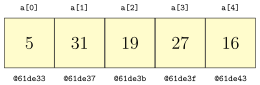
In this case, each array element is a 4-byte integer. To get the element at index 3 the compiler knows that it must be 3 × 4 = 12 bytes past the start of the array, which would be location @61de3f. Regardless of the size of the array, a similar quick computation can be used to get the value at any index. This means arrays are fast at random access, accessing a particular element anywhere in the array.
But this contiguous arrangement makes it difficult to insert and delete array elements. Suppose, for example, we want to insert the value 99 at index 2 so that the new array is [5, 99, 31, 19, 27, 16]. To make room, we have to shift most of the elements one slot to the right. This can take a while if the array is large. Moreover, how do we know we have room for another element? There is a chance that the space immediately past the end of the array is being used for something else. If that is the case, then we would have to move the array somewhere else in memory.
One way to deal with running out of room in the array when adding elements is to just make the array really large. The problem with this is how large is large enough? And we can't go around making all our arrays have millions of elements because we would be wasting a lot of memory.
Instead, what is typically done is whenever more space is needed we increase the capacity of the array by a constant factor (say by doubling it), create a new array of that size, and then copy the contents from the old array over into the new one. By doubling the capacity, we ensure that we will only periodically have to incur the expensive operation of creating a new array and moving the contents of the old one over. This type of data structure is called a dynamic array.
Implementing a dynamic array
Our implementation will have three class variables: an array a where we store all the elements, a variable capacity that is the capacity of the array, and a variable numElements that keeps track of how many elements are in the list.
For instance, consider the list [77, 24, 11]. It has three elements, so numElements is 3. However, the capacity of the list will usually be larger so that it has room for additional elements. In the figure below, we show the array with a capacity of 8. We can add five more elements before we have to increase the capacity.

The constructor
The simple constructor below sets the list to have a capacity of 100 elements and sets numElements to 0. This creates an empty list.
public AList()
{
    this.capacity = 100;
    a = new int[capacity];
    numElements = 0;
}
Getting and setting elements
Getting and setting elements of the list is straightforward.
public int get(int index)
{
    return a[index];
}

public void set(int index, int value)
{
    a[index] = value;
}
size and isEmpty
Returning the size of the list is easy since we have a variable, numElements, keeping track of the size:
public int size()
{
    return numElements;
}
Returning whether the list is empty or not is also straightforward—just return true if numElements is 0 and false otherwise. The code below does this in one line.
public boolean isEmpty()
{
    return numElements==0;
}
contains
To determine if the list contains an element or not, we can loop through the list, checking each element in turn. If we find the element we're looking for, return true. If we get all the way through the list without finding what we're looking for, then return false.
public boolean contains(int value)
{
    for (int i=0; i<numElements; i++)
        if (a[i] == value)
            return true;
    return false;
}
toString
Our toString method returns the elements of the list separated by commas and enclosed in square brackets, like [1,2,3]. The way we do this is to build up a string as we loop through the array. As we encounter each element, we add it along with a comma and a space to the string. When we're through, we have an extra comma and space at the end of the string. The final line below uses the substring method to take all of the string except for the extra comma and space and then add a closing bracket.
There is one place we have to be a little careful, and that is if the list is empty. In that case, the substring call will fail because the ending index will be negative. So we just take care of the empty list separately.
@Override
public String toString()
{
    if (numElements == 0)
        return "[]";

    String s = "[";
    for (int i=0; i<numElements; i++)
        s += a[i] + ", ";
    return s.substring(0, s.length()-2) + "]";
}
Adding and deleting things
First, we will occasionally need to increase the capacity of the list as we run out of room. We have a private method (that won't be visible to users of the class since it is only intended to be used by our methods themselves) that doubles the capacity of the list.
private void enlarge()
{
    capacity *= 2;
    int[] newArray = new int[capacity];
    for (int i=0; i<a.length; i++)
        newArray[i] = a[i];
    a = newArray;
}
To add an element to a list we first make room, if necessary. Then we set the element right past the end of the list to the desired value and increase numElements by 1.
public void add(int value)
{
    if (numElements == capacity)
        enlarge();
    a[numElements] = value;
    numElements++;
}
To delete an element from the list at a specified index we shift everything to the right of that index left by one element and reduce numElements by 1.
public void delete(int index)
{
    for (int i=index; i<numElements-1; i++)
        a[i] = a[i+1];
    numElements--;
}
Finally, we consider inserting an value at a specified index. We start, just like with add, by increasing the capacity if necessary. We then shift everything right by one element to make room for the new element. Then we add in the new element and increase numElements by 1.
public void insert(int value, int index)
{
    if (numElements == capacity)
        enlarge();

    for (int i=numElements; i>index; i--)
        a[i] = a[i-1];

    a[index] = value;
    numElements++;
}
The entire AList class
Here is the entire class.
public class AList
{
    private int[] a;
    private int numElements;
    private int capacity;

    public AList()
    {
        this.capacity = 100;
        a = new int[capacity];
        numElements = 0;
    }

    public int get(int index)
    {
        return a[index];
    }

    public void set(int index, int value)
    {
        a[index] = value;
    }

    public boolean isEmpty()
    {
        return numElements==0;
    }

    public int size()
    {
        return numElements;
    }

    public boolean contains(int value)
    {
        for (int i=0; i<numElements; i++)
            if (a[i] == value)
                return true;
        return false;
    }

    @Override
    public String toString()
    {
        if (numElements == 0)
            return "[]";

        String s = "[";
        for (int i=0; i<numElements; i++)
            s += a[i] + ", ";
        return s.substring(0,s.length()-2) + "]";
    }

    private void enlarge()
    {
        capacity *= 2;
        int[] newArray = new int[capacity];
        for (int i=0; i<a.length; i++)
            newArray[i] = a[i];
        a = newArray;
    }

    public void add(int value)
    {
        if (numElements == capacity)
            enlarge();
        a[numElements] = value;
        numElements++;
    }

    public void delete(int index)
    {
        for (int i=index; i<numElements-1; i++)
            a[i] = a[i+1];
        numElements--;
    }

    public void insert(int value, int index)
    {
        if (numElements == capacity)
            enlarge();

        for (int i=numElements; i>index; i--)
            a[i] = a[i-1];

        a[index] = value;
        numElements++;
    }
}
Using the class
Here is how we would create an object from this class and call a few of its methods:
AList list = new AList();
list.add(2);
list.add(3);
System.out.println(list.size());
Important notes
A few notes about this class (and most of the others we will develop later in the book): First, this is just the bare bones of a class whose purpose is to demonstrate how dynamic arrays work. If we were going to use this class for something important we should add some error checking. For example, the get and set methods should raise exceptions if the user were to try to get or set an index less than 0 or greater than listSize-1.
Second, after writing code for a class like this, it is important to check edge cases. For example, we should test not only how the insert method works when inserting at the middle of a list, but we should also check how it works when inserting an element at the left or right end or how insertion works on an empty list. We should also check how insert and add work when the list size bumps up against the capacity.
Last, you should probably not use this class for anything important. Java has a dynamic array class called ArrayList that you should use instead. The purpose of the class we built is to help us understand how dynamic arrays work.
Linked lists
In the dynamic array approach to lists, the key to finding an element at a specific index is that the elements of the array are laid out one after another, so we know where everything is. Each element takes up the same amount of memory and an easy computation tells how far from the start the desired element is.
The problem with this is when we insert or delete things, we have to maintain this property of array elements being all right next to each other. This can involve moving quite a few elements around. Also, once the array backing our list fills up, we have find somewhere else in memory to hold our list and copy all the elements over.
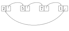
A linked list is a different approach to lists. List elements are allowed to be widely separated in memory. This eliminates the problems mentioned above for dynamic arrays, but then how do we get from one list element to the next? That's what the “link” in linked list is about. Along with each data element in the list, we also have a link, which points to where the next element in the list is located. See the figure below.
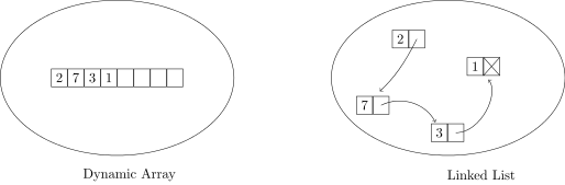
The linked list shown above is often drawn like this:
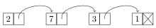
Each item in a linked list is called a node. Each node consists of a data value as well as a link to the next node in the list. The last node's link is null; in other words, it is a link going nowhere. This indicates the end of the list.
Implementing a linked list
Here is the beginning of our linked list class.
Note especially that we create a class called Node to represent a node in the list. The Node class has have two variables, one to hold the node's data, and one for the link to the next node. The tricky part here is the link is a Node object itself, so the class is self-referential.
public class LList
{
    private class Node
    {
        public int data;
        public Node next;

        public Node(int data, Node next)
        {
            this.data = data;
            this.next = next;
        }
    }

    private Node front;

    public LList()
    {
        front = null;
    }
}
There are a few things to note here. First, we have declared Node to be a nested class, a part of the LList class. This is because only the LList class needs to deal with nodes; nothing outside of the LList class needs the Node class. Secondly, notice that the class variables are declared public. We could declare them private and use getters and setters, but it's partly traditional with linked lists, and frankly a little easier, to just make Node's fields public. Since Node is such a small class and it is private to the LList class, this will not cause any problems.
The LList class actually has only one class variable, a Node object called front, which represents the first element in the list. This is all we need. If we want anything further down in the list, we just start at front and keep following links until we get where we want.
The isEmpty, size, and contains methods
Determining if the list is empty is as simple as checking whether the front of the list is set to null.
public boolean isEmpty()
{
    return front==null;
}
To find the size of the list, we walk through the list, following links and keeping count, until we get to the end of the list, which is marked by a null link.
public int size()
{
    int count = 0;
    Node n = front;
    while (n != null)
    {
        count++;
        n = n.next;
    }
    return count;
}
Determining if a value is in the list can be done similarly:
public boolean contains(int value)
{
    Node n = front;
    while (n != null)
    {
        if (n.data == value)
            return true;
        n = n.next;
    }
    return false;
}
It is worth stopping to understand how we are looping through the list, as most of the other linked list methods will use a similar kind of loop. We start at the front node and move through the list with the line n=n.next, which moves to the next element. We know we've reached the end of the list when our node is equal to null.
To picture a linked list, imagine a phone chain. Phone chains aren't in use much anymore, but the way they used to work is if school or work was canceled because of a snowstorm, the person in charge would call someone and tell them about the cancelation. That person would then call the next person in the chain and tell them. Then that person would call the next person, etc. The process of each person dialing the other person's number and calling them to tell the message is akin to the process we follow in our loops of following links.
And if we imagine that each person in the phone chain only has the next person's phone number, we have the same situation as a linked list, where each node only knows the location of the next node. This is different from arrays, where we know the location of everything. An array would be the equivalent of everyone having phone numbers in order, like 345-0000, 345-0001, 345-0002, and looping through the array would be the equivalent of having a robo-dialer call each of the numbers in order, giving the message to each person.
Getting and setting elements
Getting and setting elements at a specific index is trickier with linked lists than with dynamic list lists. To get an element we have to walk the list, link by link, until we get to the node we want. We use a count variable to keep track of how many nodes we've visited. We will know that we have reached our desired node when the count equals the desired index. Here is the get method:
public int get(int index)
{
    int count = 0;
    Node n = front;
    while (count < index)
    {
        count++;
        n = n.next;
    }
    return n.data;
}
Setting an element is similar.
public void set(int index, int value)
{
    int count = 0;
    Node n = front;
    while (count < index)
    {
        count++;
        n = n.next;
    }
    n.data = value;
}
Adding something to the front of the list
Adding an element to the front of a linked list is very quick. We create a new node that contains the value and point it to the front of the list. This node then becomes our new front, so we set front equal to it. See the figure below.

We can do this all in one line:
public void addToFront(int value)
{
    front = new Node(value, front);
}
Adding something to the back of the list
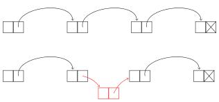
To add to the back of a linked list, we walk the list until we get to the end, create the new node, and set the end node's link to point to the new node. If the list is empty, this won't work, so we instead just set front equal to the new node. See the figure below:

Here is the code:
public void add(int value)
{
    if (front == null)
    {
        front = new Node(value, null);
        return;
    }

    Node n = front;
    while (n.next != null)
        n = n.next;
    n.next = new Node(value, null);
}
We see that adding to the front is O(1), while adding to the end is O(n). We could make adding to the end into O(1) if we have another class variable, back, that keeps track of the last node in the list. This would add a few lines of code to some of the other methods as we would occasionally need to modify the back variable.
Deleting a node
To delete a node, we reroute a link as shown below (the middle node is being deleted):
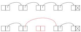
We first have to get to the node before the one to be deleted. We do this with a loop like we used for the get and set methods, except that we stop right before the deleted node. Once we get there, we can use the following line to reroute around the deleted node:
n.next = n.next.next;
This sets the current node's link to point to its neighbor's link, essentially removing its neighbor from the list. Here is the code of the method. Note the special case for deleting the first element of the list.
public void delete(int index)
{
    if (index==0)
    {
        front = front.next;
        return;
    }

    int count = 0;
    Node n = front;
    while (count < index-1)
    {
        count++;
        n = n.next;
    }
    n.next = n.next.next;
}
One other thing that is worth mentioning is that the deleted node is still there in memory but we don't have any way to get to it, so it is essentially gone and forgotten about. Eventually Java's garbage collector will recognize that nothing is pointing to it and recycle its memory for future use.
Inserting a node
To insert a node, we first create the node to be inserted and then reroute a link to put it into the list. The rerouting code is very similar to what we did for deleting a node. Here is how the rerouting works:
To do the insertion, we first loop through the list to get to the place to insert the link. This is just like what we did for the delete method. We can create the new node and reroute in one line:
n.next = new Node(value, n.next);
Here is the code for the insert method.
public void insert(int index, int value)
{
    if (index == 0)
    {
        front = new Node(value, front);
        return;
    }

    int count = 0;
    Node n = front;
    while (count < index-1)
    {
        count++;
        n = n.next;
    }
    n.next = new Node(value, n.next);
}
The entire LList class
Here is the entire linked list class:
public class LList
{
    private class Node
    {
        public int data;
        public Node next;

        public Node(int data, Node next)
        {
            this.data = data;
            this.next = next;
        }
    }

    private Node front;

    public LList()
    {
        front = null;
    }

    public boolean isEmpty()
    {
        return front==null;
    }

    public int size()
    {
        int count = 0;
        Node n = front;
        while (n != null)
        {
            count++;
            n = n.next;
        }
        return count;
    }

    public int get(int index)
    {
        int count = 0;
        Node n = front;
        while (count < index)
        {
            count++;
            n = n.next;
        }
        return n.data;
    }

    public void set(int index, int value)
    {
        int count = 0;
        Node n = front;
        while (count < index)
        {
            count++;
            n = n.next;
        }
        n.data = value;
    }

    public boolean contains(int value)
    {
        Node n = front;
        while (n != null)
        {
            if (n.data == value)
                return true;
            n = n.next;
        }
        return false;
    }

    @Override
    public String toString()
    {
        if (front == null)
            return "[]";

        Node n = front;
        String s = "[";
        while (n != null)
        {
            s += n.data + ", ";
            n = n.next;
        }
        return s.substring(0, s.length()-2) + "]";
    }

    public void add(int value)
    {
        if (front == null)
        {
            front = new Node(value, null);
            return;
        }

        Node n = front;
        while (n.next != null)
            n = n.next;
        n.next = new Node(value, null);
    }

    public void addToFront(int value)
    {
        front = new Node(value, front);
    }

    public void delete(int index)
    {
        if (index == 0)
        {
            front = front.next;
            return;
        }

        int count = 0;
        Node n = front;
        while (count < index-1)
        {
            count++;
            n = n.next;
        }
        n.next = n.next.next;
    }

    public void insert(int index, int value)
    {
        if (index == 0)
        {
            front = new Node(value, front);
            return;
        }

        int count = 0;
        Node n = front;
        while (count < index-1)
        {
            count++;
            n = n.next;
        }
        n.next = new Node(value, n.next);
    }
}
Using the class
Here is how we would create an object from this class and call a few of its methods. This is essentially the same code as we tested the dynamic array class with. Remember that linked lists and dynamic arrays are two ways of implementing the same data structure, a list.
LList list = new LList();
list.add(2);
list.add(3);
System.out.println(list.size());
Working with linked lists
There are a number of exercises at the end of this chapter that ask you to write additional methods for the linked list class. These are particularly useful exercises for becoming comfortable working with linked lists. Here are a few helpful hints for working on them.
Basics
First, remember the basic idea of a linked list, that each item in the list is a node that contains a data value and a link to the next node in the list. Creating a new node is done with a line like below:
Node n = new Node(19, null);
This creates a node with value 19 and a link that points to nothing. Suppose we want to create a new node that points to another node in the list called m. Then we would do the following:
Node n = new Node(19, m);
To change the link of n to point to something else, say the front of the list, we could do the following:
n.next = front;
Remember that the front marker is a Node variable that keeps track of which node is at the front of the list.
Looping
To move through a linked list, a loop like below is used:
Node n = front;
while (n != null)
    n = n.next;
This will loop through the entire list. We could use a counter if we just want to loop to a certain index in the list, like below (looping to index 10):
Node n = front;
int count = 0;
while (count < 10)
{
    count++;
    n = n.next;
}
Using pictures
Many linked list methods just involve creating some new nodes and moving some links around. To keep everything straight, it can be helpful to draw a picture. For instance, below is the picture we used earlier when describing how to add a new node to the front of a list:
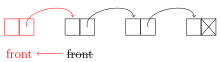
And we translated this picture into the following line:
public void addToFront(int value)
{
    front = new Node(value, front);
}
This line does a few things. It creates a new node, points that node to the old front of the list, and moves the front marker to be at this new node.
Edge cases
When working with linked lists, as with many other things, it is important to worry about edge cases. These are special cases like an empty list, a list with one element, deleting the first or last element in a list, etc. Often with linked list code, one case will handle almost everything except for one or two special edge cases that require their own code.
For instance, as we saw earlier, to delete a node from a list, we loop through the list until we get to the node right before the node to be deleted and reroute that node's link around the deleted node. But this won't work if we are deleting the first element of the list. So that's an edge case, and we need a special case to handle that. Here again is the code for the delete method:
public void delete(int index)
{
    // edge case for deleting the first element
    if (index == 0)
    {
        front = front.next;
        return;
    }

    // This is the code for deleting any other element
    int count = 0;
    Node n = front;
    while (count < index-1)
    {
        count++;
        n = n.next;
    }
    n.next = n.next.next;
   }
Null pointer exceptions
When working with nodes, there is a good chance of making a mistake and getting a NullPointerException from Java. This usually happens if you use an object without first initializing it. For example, the following will cause a null pointer exception:
Node myNode;

// some code not involving myNode might go here

if (myNode.value == 3)
    // some more code goes here...
The correction is to either set myNode equal to some other Node object or initialize it like below:
Node myNode = new Node(42, null);
In summary, if you get a null pointer exception, it usually indicates an object that has been declared but not initialized.
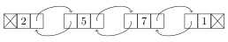
Doubly- and circularly-linked lists
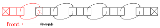
There are a couple of useful variants on linked lists. The first is a circularly-linked list is one where the link of the last node in the list points back to the start of the list, as shown below.
Working with circularly-linked lists is similar to working with ordinary ones except that there's no null link at the end of the list (you might say the list technically has no start and no end, just being a continuous loop). One thing to do if you need to access the “end” of the list is to loop until node.next equals front. However, a key advantage of a circularly-linked list is that you can loop over its elements continuously.
The second variant of a linked list is a doubly-linked list, where each node has two links, one to the next node and one to the previous node, as shown below:
Having two links can be useful for methods that need to know the predecessor of a node or for traversing the list in reverse order. Doubly-linked lists are a little more complex to implement because we now have to keep track of two links for each node. To keep track of all the links, it can be helpful to sketch things out. For instance, here is a sketch useful for adding a node to the front of a doubly-linked list.
We see from the sketch that we need to create a new node whose next link points to the old front and whose prev link is null. We also have to set the prev link of the old front to point to this new node, and then set the front marker to the new node. A special case is needed if the list is empty.
Comparison of dynamic arrays and linked lists
First, let's look at running times of the methods. Let n denote the size of the list.
- Getting/setting a specific index
Dynamic array — O(1). Getting and setting both consist of a single array operation, which translates to a quick memory address calculation at the machine level. The size of the list has no effect on the calculation.
Linked list — O(n). To get or set a specific index requires us to follow links until we get to the desired index. In the worst case, we have to go through all n links (when the index is the end of the list), and on average we have to go through n/2 links.
-
isEmptyDynamic array — O(1). We just check if the class variable
numElementsis 0 or not.Linked list — O(1). We just check if the class variable
frontis equal tonullor not. -
sizeDynamic array — O(1). We just return the value of the class variable
numElements.If we did not have that class variable, then it would be an O(n) operation because we would have to loop through and count how many elements there are. The tradeoff here is that the
insert,delete, andaddmethods have to updatenumElementseach time they are called, adding a little bit of time to each of them. Essentially, by having the class variable, we have spread out thesizemethod's work over all those other methods.Linked list — O(n). Our code must loop through the entire list to count how many elements there are. On the other hand, we could make this O(1) by adding a class variable
numElementsto the list and updating it whenever we add or delete elements, just like we did for our dynamic array class. -
containsDynamic array — O(n). Our code searches through the list, element-by-element, until it finds what it's looking for or gets to the end of the list. If the desired value is at the end of the list, this will take n steps. On average, it will take n/2 steps.
Linked list — O(n). Our linked-list code behaves similarly to the dynamic list code.
- Adding and deleting elements
Dynamic array — First, increasing the capacity of the list is an O(n) operation, but this has to be done only rarely. The rest of the
addmethod is O(1). So overall, adding is said to be amortized O(1), which is to say that most of the time it adding is an O(1) operation, but it can on rare occasions be O(n).On the other hand, inserting or deleting an element in the middle of the list is O(n) on average because we have to move around big chunks of the array either to make room or to make sure the elements stay contiguous.
Linked list — The actual operation of inserting or deleting a node is an O(1) operation as it just involves moving around a link and creating a new node (when inserting). However, we have to walk through the list to get to the location where the insertion or deletion happens, and this takes O(n) operations on average. So, the way we've implemented things, a single insert or delete will run in O(n) time.
However, once you're at the proper location, inserting or deleting is very quick. Consider a
removeAllmethod that removes all occurrences of a specific value. To implement this we could walk through the list, deleting each occurrence of the value as we encounter it. Since we are already walking through the list, no further searching is needed to find a node and the deletions will all be O(1) operations. SoremoveAllwill run in O(n) time.Also, inserting or deleting at the front of the list is an O(1) operation as we don't have to go anywhere to find the front. And, as noted earlier, adding to a list is currently O(n) because we have to walk through the entire list to get there, but it can be made into O(1) operation if we add another class variable to keep track of the end of the list.
In terms of which is better—dynamic arrays or linked lists—there is no definite answer as they each have their uses. In fact, for most applications either will work fine. For applications where speed is critical, dynamic arrays are better when a lot of random access is involved, whereas linked lists can be better when it comes to insertions and deletions. In terms of memory usage, either one is fine for most applications. For really large lists, remember that linked lists require extra memory for all the links, an extra five or six bytes per list element. Dynamic arrays have their own potential problems in that not every space allocated for the array is used, and for really large arrays, finding a contiguous block of memory could be tricky.
We also have to consider cache performance. Not all RAM is created equal. RAM access can be slow, so modern processors include a small amount cache memory that is faster to access than regular RAM. Arrays, occupying contiguous chunks of memory, generally give better cache performance than linked lists whose nodes can be spread out in memory. Chunks of the array can be copied into the cache, making it faster to iterate through a dynamic array than a linked list.
Making the linked list class generic
The linked list class we created in this chapter works only for integer lists. We could modify it to work with strings by going through and replacing the int declarations with String declarations, but that would be tedious. And then if we wanted to modify it to work with doubles or longs or some object, we would have to do the same tedious replacements all over again. It would be nice if we could modify the class once so that it works with any type. This is where Java's generics come in.
The process of making a class work with generics is pretty straightforward. We will add a little syntax to the class to indicate we are using generics and then replace the int declarations with T declarations. The name T, short for “type,” acts as a placeholder for a generic type. (You can use other names instead of T, but the T is somewhat standard.)
First, we have to introduce the generic type in the class declaration:
public class LList<T>
The slanted brackets are used to indicate a generic type. After that, the only thing we have to do is anywhere we refer to the data type of the values stored in the list, we have to change it from int to T. For example, the get method changes as shown below:
public int get(int index)                  public T get(int index)
{                                          {
    int count = 0;                           int count = 0;
    Node n = front;                          Node n = front;
    while (count < index)                    while (count < index)
    {                                        {
        count++;                                 count++;
        n = n.next;                              n = n.next;
    }                                        }
    return n.data;                           return n.data;
}                                         }
Notice that the return type of the method is now type T instead of int. Notice also that index stays an int. Indices are still integers, so they don't change. It's only the data type stored in the list that changes to type T.
One other small change is that when comparing generic types, using == doesn't work anymore, so we have to replace that with a call to .equals(), just like when comparing strings in Java.
Here is the entire class:
public class LList<T>
{
    private class Node
    {
        public T data;
        public Node next;

        public Node(T data, Node next)
        {
            this.data = data;
            this.next = next;
        }
    }

    private Node front;

    public LList()
    {
        front = null;
    }

    public boolean isEmpty()
    {
        return front==null;
    }

    public int size()
    {
        int count = 0;
        Node n = front;
        while (n != null)
        {
            count++;
            n = n.next;
        }
        return count;
    }

    public T get(int index)
    {
        int count = 0;
        Node n = front;
        while (count < index)
        {
            count++;
            n = n.next;
        }
        return n.data;
    }

    public void set(int index, T value)
    {
        int count = 0;
        Node n = front;
        while (count < index)
        {
            count++;
            n = n.next;
        }
        n.data = value;
    }

    public boolean contains(T value)
    {
        Node n = front;
        while (n != null)
        {
            if (n.data.equals(value))
                return true;
            n = n.next;
        }
        return false;
    }

    @Override
    public String toString()
    {
        if (front == null)
            return "[]";

        Node n = front;
        String s = "[";
        while (n != null)
        {
            s += n.data + ", ";
            n = n.next;
        }
        return s.substring(0, s.length()-2) + "]";
    }

    public void add(T value)
    {
        if (front == null)
        {
            front = new Node(value, null);
            return;
        }

        Node n = front;
        while (n.next != null)
            n = n.next;
        n.next = new Node(value, null);
    }

    public void addToFront(T value)
    {
        front = new Node(value, front);
    }

    public void delete(int index)
    {
        if (index == 0)
        {
            front = front.next;
            return;
        }

        int count = 0;
        Node n = front;
        while (count < index-1)
        {
            count++;
            n = n.next;
        }
        n.next = n.next.next;
    }

    public void insert(int index, T value)
    {
        if (index == 0)
        {
            front = new Node(value, front);
            return;
        }

        int count = 0;
        Node n = front;
        while (count < index-1)
        {
            count++;
            n = n.next;
        }
        n.next = new Node(value, n.next);
    }
}
Here is an example of the class in action:
LList<String> list = new LList<String>();
list.add("first");
list.add("second");
System.out.println(list);
And the output is
[first, second]
The Java Collections Framework
While it is instructive to write our own list classes, it is best to use the ones provided by Java for most practical applications. Java's list classes have been extensively tested and optimized, whereas ours are mostly designed to help us understand how the two types of lists work. On the other hand, it's nice to know that if we need something slightly different from what Java provides, we could code it.
Java's Collections Framework contains, among many other things, an interface called List. There are two classes implementing it: a dynamic array class called ArrayList and and a linked list class called LinkedList.
Here are some sample declarations:
List<Integer> list = new ArrayList<Integer>();
List<Integer> list = new LinkedList<Integer>();
The Integer in the slanted braces indicates the data type that the list will hold. This is an example of Java generics. We can put any class name here. Here are some examples of other types of lists we could have:
List<String> | list of strings |
List<Double> | list of doubles |
List<Card> | list of Card objects (assuming you've created a Card class) |
List<List<Integer>> | list of integer lists |
List methods
Here are the most useful methods of the List interface. They are available to both ArrayLists and LinkedLists.
| Method | Description |
|---|---|
add(x) | adds x to the list |
add(i,x) | adds x to the list at index i |
contains(x) | returns whether x is in the list |
equals(a) | returns whether the list equals a |
get(i) | returns the value at index i |
indexOf(x) | returns the first index (location) of x in the list |
isEmpty() | returns whether the list is empty |
lastIndexOf(x) | like indexOf, but returns the last index |
remove(i) | removes the item at index i |
remove(x) | removes the first occurrence of the object x |
removeAll(x) | removes all occurrences of x |
set(i,x) | sets the value at index i to x |
size() | returns the number of elements in the list |
subList(i,j) | returns a slice of a list from index i to j-1, sort of like substring |
Methods of java.util.Collections
There are some useful static Collections methods that operate on lists (and, in some cases, other Collections objects that we will see later):
| Method | Description |
|---|---|
addAll(a, x1,..., xn) | adds x1, x2, …, xn to the list a |
binarySearch(a,x) | returns whether x is in the collection a |
frequency(a,x) | returns a count of how many times x occurs in a |
max(a) | returns the largest element in a |
min(a) | returns the smallest element in a |
replaceAll(a,x,y) | replaces all occurrences of x in a with y |
reverse(a) | reverses the elements of a |
rotate(a,n) | rotates all the elements of a forward n positions |
shuffle(a) | puts the contents of a in a random order |
sort(a) | sorts the collection a |
swap(a,i,j) | swaps elements at indices i and j |
Applications of lists
It's hard to write a program of any length that doesn't use lists (or arrays) somewhere. Lists of names, words, numbers, and so on are so common in everyday life that its no surprise that they show up in programs. Later in this chapter there is an exercise about some practical applications of lists.
One exercise in particular demonstrates the usefulness of lists. Here is the statement of the problem:
Write a program that asks the user to enter a length in feet. The program should then give the user the option to convert from feet into inches, yards, miles, millimeters, centimeters, meters, or kilometers. Say if the user enters a 1, then the program converts to inches, if they enter a 2, then the program converts to yards, etc.
While this could certainly be written using if statements or a switch statement, if there are a lot of conversions to make, the code will be long and messy. The code can be made short and elegant by storing all the conversion factors in a list. This would also make it easy to add new conversions as we would just have to add some values to the list, as opposed to copying and pasting chunks of code. Moreover, the conversion factors could be put into a file and read into the list, meaning that the program itself need not be modified at all. This way, our users (who may not be programmers) could easily add conversions.
This is of course a really simple example, but it hopefully demonstrates the main point—that lists can eliminate repetitious code and make programs easier to maintain.
Iterators*
This section can be skipped. It is about how to make a class work with Java's foreach loop.Lists in Java support a short type of for loop called a foreach loop that works as follows:
for (Integer x: list)
    System.out.println(x);
We can add this feature to our own classes, like our linked list class. To start, we need the following import statement.
import java.util.Iterator;
Next, our class needs to implement the Iterable interface.
public class LList<T> implements Iterable<T>
We then create a private nested class that tells how to traverse the list. This class implements the Iterator interface. It must have methods hasNext, next, and remove. Its code is shown below.
private class LListIterator implements Iterator<T>
{
    private Node location;

    public LListIterator(LList<T> d)
    {
        location = front;
    }

    public T next()
    {
        T value = location.data;
        location = location.next;
        return value;
    }

    public boolean hasNext()
    {
        return location!=null;
    }

    public void remove() {}
}
There is a class variable called location that keeps track of where in the list we are. The constructor sets up the iterator and starts it at the front of the list. The next method returns the next element in the list and advances the iterator. The hasNext method returns true or false depending on whether there is anything left in the list to be iterated over. To do this, we just check if location is null. The remove method is part of the interface, so we must include it, but we have decided not to do anything with it.
The one other thing we need is a method to create the iterator:
public Iterator<T> iterator()
{
    return new LListIterator(this);
}
So, just add all this to the linked list class and we can then iterate through it using the foreach loop, like below:
LList<Integer> list = new LList<Integer>();

list.add(2);
list.add(3);

for (Integer x : list)
    System.out.println(x);
Exercises
- Add the following methods to the dynamic array class from this chapter.
-
addAll(a)— Adds all the elements of the arrayato the end of the list. -
addSorted(x)— Assuming the list is in sorted order, this method addsxto the list in the appropriate place so that the list remains sorted. -
allIndicesOf(x)— Returns an integer ArrayList consisting of every index in the list wherexoccurs. -
clear()— Empties all the elements from the list. -
count(x)— Returns the number of occurrences ofxin the list. -
equals(L)— Returnstrueif the list is equal toLandfalseotherwise. Lists are considered equal if they have the same elements in the same order. -
indexOf(x)— Returns the first index ofxin the list and -1 ifxis not in the list. -
lastIndexOf(x)— Returns the last index ofxin the list and -1 ifxis not in the list. -
remove(x)— Removes the first occurrence ofxfrom the list. -
removeAll(x)— Removes all occurrences ofxfrom the list. -
removeDuplicates()— Removes all duplicate items from the list so that each element in the list occurs no more than once -
reverse()— Reverses the elements of the list -
rotate()— Shifts the elements of the list so that the last item in the list is now first and everything else is shifted right by one position. -
rotate(n)— Like above but every elements shifts forward bynunits. -
sublist(i,j)— Returns a new list consisting of the elements of the original list starting at indexiand ending at indexj-1.
-
- Add the methods of the previous problem to the linked list class. Try to implement them as efficiently as possible, creating as few new nodes as possible and instead relying on moving around links. Use as few loops as possible and do them without calling other methods we wrote for the class.
- Add the following methods to the linked list class. These methods should just be done using a single while loop without calling any other methods we wrote for the class.
-
simplify()— removes any consecutive occurrences of the same value, replacing them with just a single occurrence of that value. For instance if the list is[1,3,3,4,5,5,6,1,1,3,7,7,7,7,8], thenlist.simplify()should turn the list into[1,3,4,5,6,1,3,7,8]. Note that the method should modify the list and should not return anything. -
onlyKeepEvenIndices()— modifies the list so that only the elements at even indices are left in the list. For instance, if the list is[1,3,4,5,7,8,9], thenlist.onlyKeepEvenIndices()should modify the list into[1,4,7,9]. -
doubler()— modifies the list so that each element is replaced by two adjacent copies of itself. For instance, if the list is[1,2,3,3,4], thenlist.doubler()should modify the list into[1,1,2,2,3,3,3,3,4,4].
-
- Add the following methods to the linked list class.
-
removeZeroes()— removes all the zeroes from the list. This should run in O(n) time and should use O(1) additional space. -
combine(list2)— adds all of the items of the LList objectlist2to the end of the current list. For instance, iflist = [1,2,3],list2 = [4,5,6], and we calllist.combine(list2), thenlistshould equal[1,2,3,4,5,6]after the method call.You should do this without creating any new nodes, except perhaps one to use to traverse a list. In particular, this means that you can't use append or insert because they create new nodes. The combining must be done just by manipulating links.
-
evenToString()— This method should behave like thetoStringmethod we wrote for theLListclass, except that it returns a string containing only the elements at even indices. For instance, if the list is[1,3,4,5,7,8,9], thenlist.evenToString()should return"[1,4,7,9]".
-
- Add a field called
backto theLListclass that keeps track of the back of the list. To do this properly, you will have to modify many of the methods to keep track of the new field. - Implement a circularly-linked list, giving it the same methods as the
LListclass. - Add a method called
rotateto the circularly linked list class. This method should rotate all the elements to the left by one unit, with the end of the list wrapping around to the front. For instance,[1,2,3,4]should become[2,3,4,1]. Your solution to this part must run in O(1) time. - Implement a doubly-linked list, giving it the same methods as the
LListclass. - Add a method called
reverseToString()to the doubly-linked list class. It should return a string containing the list elements in reverse order. - Rewrite the doubly-linked list class to include a field called
backthat keeps track of the back of the list. To do this properly, you will have to modify many of the methods to keep track of the new field. - Implement a circularly-doubly-linked list, giving it the same methods as the
LListclass. - Add the methods of problems 1-4 to the doubly-linked list class.
- Add the methods of problems 1-4 to the circularly-doubly-linked class.
- Use lists from the Collections Framework to do the following:
- Write a method
primesthat takes an integernand returns a list of all the primes less than or equal ton. - Write a method called
mergethat takes two sorted lists and merges them together into a single, sorted list. - Write a program that asks the user to enter a length in feet. The program should then give the user the option to convert from feet into inches, yards, miles, millimeters, centimeters, meters, or kilometers. Say if the user enters a
1, then the program converts to inches, if they enter a2, then the program converts to yards, etc. While this can be done with if statements, it is much shorter with lists and it is also easier to add new conversions if you use lists. - Write a method that takes and list
listcontaining integers between 1 and 100 and returns a new list whose first element is how many ones are inlist, whose second element is how many twos are inlist, etc. - Write a method
getRandomthat takes a list and returns a random element from the list. - Write a method
sample(list, n)that returns a list ofnrandom elements fromlist. - Write a method
breakIntoTeamsthat takes a list containing an even number of people's names, randomly breaks all the people into teams of two, and returns a list of the teams. - Write a program that estimates the average number of drawings it takes before the user's numbers are picked in a lottery that consists of correctly picking six different numbers that are between 1 and 10. To do this, run a loop 1000 times that randomly generates a set of user numbers and simulates drawings until the user's numbers are drawn. Find the average number of drawings needed over the 1000 times the loop runs.
- Write a program that simulates drawing names out of a hat. In this drawing, the number of hat entries each person gets may vary. Allow the user to input a list of names and a list of how many entries each person has in the drawing, and print out who wins the drawing.
- Write a method
runLengthEncodethat performs run-length encoding on a list. It should return a list consisting of all lists of the form[x,n], wherexis an element from the list andnis its frequency. For example, the encoding of the list[a,a,b,b,b,b,c,c,c,d]is[[2,a],[4,b],[3,c],[1,d]]. - Write a simple quiz program that reads a bunch of questions and answers from a file and randomly chooses five questions. It should ask the user those questions and print out the user's score.
- Write a method
- Add exception-handling to the
AListclass. The class should throw exceptions if the user tries to access an index outside of the list.
Stacks and Queues
This chapter is about two of the simplest and most useful data structures—stacks and queues. Stacks and queues behave like lists of items, each with its own rules for how items are added and removed.
Stacks
A stack is a LIFO structure, short for last in, first out. Think of a stack of dishes, where the last dish placed on the stack is the first one to be taken off. Or as another example, think of a discard pile in a game of cards where the last card put on the pile is the first one to be picked. Stacks have two main operations: push and pop. The push operation puts a new element on the top of the stack and the pop element removes an element from the top of the stack and returns it to the caller.
To demonstrate how a stack works, suppose we have a stack of integers. Say we push 1, 2, and 3 onto the stack, then do a pop operation, then push 4 onto the stack. The stack will grow as follows, where the left side of each list is the “top” of the stack:

Queues
A queue is a FIFO structure, short for first in, first out. A queue is like a line (or queue) at a store. The first person in line is the first person to check out. If a line at a store were implemented as a stack, on the other hand, the last person in line would be the first to check out, which would lead to lots of angry customers. Queues have two main operations, enqueue and dequeue. The enqueue operation adds a new element to the back of the queue, and the dequeue operation removes the element at the front of the queue and returns it to the caller.
To demonstrate a queue, let's enqueue 1, 2, and 3, then dequeue, and finally enqueue 4. The queue grows as follows, where the left side of each list is the “front” of the queue:

Deques
There is one other data structure, called a deque, that we will mention briefly. It behaves like a list that supports adding and removing elements on either end. The name deque is short for double-ended queue. Since it supports addition and deletion at both ends, it can also be used as a stack or a queue. One of the exercises at the end of this chapter is about implementing a deque class.
Implementing a stack class
Our class will have a push method that puts an item on the top of the stack and a pop method that removes and returns the value of the top item on the stack. It will also have a peek method, which returns the value of the top item without removing it from the stack, and an isEmpty method.
We implement the stack as a linked list. The class will have an inner class called Node, just like with linked lists. We will have one class variable, a node called top to keep track of what is at the top of the stack. The constructor sets it to null, so we start with an empty stack. Also, we will use generics to allow us to use any data type with our stack. Here is the start of the class:
public class LLStack<T>
{
    private class Node
    {
        public T data;
        public Node next;

        public Node(T data, Node next)
        {
            this.data = data;
            this.next = next;
        }
    }

    private Node top;

    public LLStack()
    {
        top = null;
    }
The isEmpty and peek methods
The isEmpty method is nearly the same as it is for linked lists:
public boolean isEmpty()
{
    return top==null;
}
The peek method is also very short as we just have to return the data value stored at the top of the stack.
public T peek()
{
    return top.data;
}
The method also should make sure that the stack is not empty and raise an exception if it is, but for simplicity, we will not do that.
Pushing and popping things
Pushing things onto and popping things off of the stack is a matter of moving around links and where the top variable points to. To push an item onto the stack, we create a new node for it that points to the current top and then change the top variable to point to the new node. This very similar to the addToFront method for a linked list, and it can be done in one line:
public void push(T value)
{
    top = new Node(value, top);
}
See the figure below:
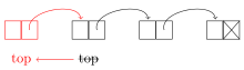
To pop an item from the stack, we have to both return the value of the item and delete it. To delete the top item, we set top equal to top.next. This points the top variable to the second item from the top (or null if there is only one element). But before we do this, we save the value of the old top item so we can later return it.
public T pop()
{
    T data = top.data;
    top = top.next;
    return data;
}
See the figure below:
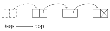
Here is the entire stack class:
public class LLStack<T>
{
    private class Node
    {
        public T data;
        public Node next;

        public Node(T data, Node next)
        {
            this.data = data;
            this.next = next;
        }
    }

    private Node top;

    public LLStack()
    {
        top = null;
    }

    public boolean isEmpty()
    {
        return top==null;
    }

    public T peek()
    {
        return top.data;
    }

    public void push(T value)
    {
        top = new Node(value, top);
    }

    public T pop()
    {
        T data = top.data;
        top = top.next;
        return data;
    }
}
Here is a short demonstration of the class in use:
LLStack<Integer> stack = new LLStack<Integer>();
stack.push(3);
stack.push(4);
stack.push(5);
System.out.print(stack.pop() + " " + stack.pop() + " " + stack.pop());
5 4 3
Finally, it is worth noting that all of the methods are O(1).
Implementing a queue class
Our queue class will have an enqueue method that puts an item at the back of the queue and a dequeue method that removes and returns the item at the front of the queue. It will also have isEmpty and peek methods. Like with stacks, we will implement the queue as a linked list. Here we have two variables, front and back, to keep track of the two ends of the queue. The constructor sets both to null, so we start with an empty queue. Other than that, the queue class starts out quite similarly to the stack class. Here is the start of the class:
public class LLQueue<T>
{
    private class Node
    {
        public T data;
        public Node next;

        public Node(T data, Node next)
        {
            this.data = data;
            this.next = next;
        }
    }

    private Node front;
    private Node back;

    public LLQueue()
    {
        front = back = null;
    }
Queue methods
The peek and isEmpty methods are practically the same as for stacks. We just use front in place of top.
Just like with stacks, adding and removing things with queues comes down to rearranging a few links and whatnot.
To enqueue something we create a new node for it and place it at the back of the queue by setting the current back.next to point to the new node. We then set back equal to the new node. See the figure below:
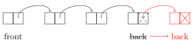
There is an edge case we have to consider, which is if the queue is empty. In that case, setting back.next would raise a null pointer exception, so instead we just set back equal to the new node. We also have to set front to that new node because there is only one node and it is at both the back and the front of the queue. Here is the code:
public void enqueue(T value)
{
    Node newNode = new Node(value, null);
    if (front==null)
        front = back = newNode;
    else
        back = back.next = newNode;
}
To dequeue we return the value of front.data and set front to front.next, as shown below:
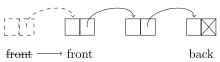
The edge case we have to worry about here is if this operation empties the list. In that case, we've deleted the back of the list and so we update back to null. Here is the code:
public T dequeue()
{
    T data = front.data;
    front = front.next;
    if (front==null)
        back = null;
    return data;
}
Here is the entire class:
public class LLQueue<T>
{
    private class Node
    {
        public T data;
        public Node next;

        public Node(T data, Node next)
        {
            this.data = data;
            this.next = next;
        }
    }

    private Node front;
    private Node back;

    public LLQueue()
    {
        front = back = null;
    }

    public boolean isEmpty()
    {
        return front==null;
    }

    public T peek()
    {
        return front.data;
    }

    public void enqueue(T value)
    {
        Node newNode = new Node(value, null);
        if (front==null)
            front = back = newNode;
        else
            back = back.next = newNode;
    }

    public T dequeue()
    {
        T data = front.data;
        front = front.next;
        if (front==null)
            back = null;
        return data;
    }
}
Here is an example of the class in action.
LLQueue<Integer> queue = new LLQueue<Integer>();
queue.enqueue(3);
queue.enqueue(4);
queue.enqueue(5);
System.out.println(queue.dequeue() + " " + queue.dequeue() + " " + queue.dequeue());
3 4 5
Finally, just like with stacks, it is worth noting that all of the queue methods are O(1).
Stacks, queues, and deques in the Collections Framework
The Collections Framework supports all three of these data structures. According to Java's documentation, all three are best implemented using the ArrayDeque class, which is kind of a workhorse class, able to implement a variety of data structures.
Stacks
The Collections Framework contains a Stack interface, but it is old and flawed and only kept around to avoid breaking old code. The Java documentation recommends against using it. Instead, it recommends using the Deque interface, which is usually implemented by the ArrayDeque class.
Using this, we have the expected push, pop methods. The peek method is called element. Here is a simple example:
import java.util.ArrayDeque;
import java.util.Deque;

public class StackExample
{
    public static void main(String[] args)
    {
        Deque<Integer> stack = new ArrayDeque<Integer>();
        stack.push(3);
        stack.push(4);
        stack.push(5);
        stack.pop();
        stack.push(6);
        System.out.println(stack);
    }
}
[6, 4, 3]
The top of the stack here is on the left.
Queues
For queues, there is an interface called Queue which we usually implement with the ArrayDeque class. The queue's enqueue and dequeue operations are called add and remove, and its peek operation is called element. Here is a simple example:
import java.util.ArrayDeque;
import java.util.Queue;

public class QueueExample
{
    public static void main(String[] args)
    {
        Queue<Integer> queue = new ArrayDeque<Integer>();
        queue.add(3);
        queue.add(4);
        queue.add(5);
        queue.remove();
        queue.add(6);
        System.out.println(queue);
    }
}
[4, 5, 6]
The front of the queue here is on the left.
Deques
We use the Deque interface for deques in the Collections Framework and implement it using the ArrayDeque class. The class has the following methods:
-
addFirst— add something to the beginning of the list. -
addLast— add something to the end of the list. -
getFirst— returns the first element of the list without removing it. -
getLast— returns the last element of the list without removing it. -
removeFirst— removes the first thing from list. -
removeLast— removes the last thing from list.
Here is an example:
import java.util.ArrayDeque;
import java.util.Deque;

public class DequeExample
{
    public static void main(String[] args)
    {
        Deque<Integer> deque = new ArrayDeque<Integer>();
        deque.addFirst(3);
        deque.addFirst(4);
        deque.addFirst(5);
        deque.addLast(10);
        deque.addLast(11);
        deque.removeLast();
        deque.removeFirst();
        System.out.println(deque);
    }
}
[4, 3, 10]
The front of the deque here is on the left.
More about using the Collections Framework
Each of the three data structures can also be implemented using the LinkedList class, though Java's documentation says that ArrayDeque is faster.
The ArrayDeque class and LinkedList classes contain a number of other methods like isEmpty, size and contains and remove that may be useful.
Finally, all of the methods mentioned—pop, remove, element etc.—will raise an exception if they fail (like trying to pop from an empty stack). There are other methods provided by the ArrayDeque and LinkedList classes that behave the same as these except that instead of raising an exception, they will return false or null upon failure. For example, the non-exception-raising equivalents for queues of add, remove, and element are offer, poll, and peek. See the Java documentation for further details.
Applications
Stacks and queues have many applications in algorithms and the architecture of computers. Here are a few.
- Breadth-first search/Depth-first search — These are useful searching algorithms that are discussed in this section. They can be implemented with nearly the same algorithm, the only major change being that breadth-first search uses a queue, whereas depth-first search uses a stack.
- Queues are used in operating systems for scheduling tasks. Often, if the system is busy doing something, tasks will pile up waiting to be executed. They are usually done in the order in which they are received, and so a queue is an appropriate data structure to handle this.
- Most programming languages use a call stack to handle function calls. When a program makes a function call, it needs to store information about where in the program to return to after the function is done as well as reserve some memory for local variables. The call stack is used for these things. To see why a stack is used, suppose the main program P calls function A which in turn calls function B. Once B is done, we need to return to A, which was the most recent function called before B. Since we always need to go back to the most recent function, a stack is appropriate. The call stack is important for recursion, as we will see in the recursion chapter.
- Stacks are useful for parsing formulas. Suppose, for example, we need to write a program to evaluate user-entered expressions like 2*(3+4)+5*6. One technique is to convert the expression into what is called postfix notation (or Reverse Polish notation) and then use a stack. In postfix, an expression is written with its operands first followed by the operators. Ordinary notation, with the operator between its operands, is called infix notation.
For example, 1+2 in infix becomes 1 2 + in postfix. The expression 1+2+3 becomes 1 2 3 + +, and the expression (3+4)*(5+6) becomes 3 4 + 5 6 + *.
To evaluate a postfix expression, we use a stack of operands and results. We move through the formula left to right. Every time we meet an operand, we push it onto the stack. Every time we meet an operator, we pop the top two items from the stack, apply the operand to them, and push the result back onto the stack.
For example, let's evaluate (3+4)*(5+6), which is 3 4 + 5 6 + * in postfix. Here is the sequence of operations.
3 push it onto stack. Stack = [3]4 push it onto stack. Stack = [4, 3]+ pop 4 and 3 from stack, compute 3+4=7, push 7 onto stack. Stack = [7]5 push it onto stack. Stack = [5, 7]6 push it onto stack. Stack = [6, 5, 7]+ pop 6 and 5 from stack, compute 5+6=11, push 11 onto stack. Stack = [11, 7]* pop 11 and 7 from stack, compute 7*11=77, push 77 onto stack Stack = [77]The result is 77, the only thing left on the stack at the end.
Postfix notation has some benefits over infix notation in that parentheses are never needed and it is straightforward to write a program to evaluate postfix expressions. In fact, many calculators of the '70s and '80s used postfix for just this reason. Calculator users would enter their formulas using postfix notation. To convert from infix to postfix there are several algorithms. A popular one is Dijkstra's Shunting Yard Algorithm. It uses stacks as a key part of what it does.
In general, queues are useful when things must be processed in the order in which they were received, and stacks are useful if things must be processed in the opposite order, where the most recent thing must be processed first.
Exercises
- The following sequence of stack operations is performed. What does the stack look like after all the operations have been performed? Please indicate where the stack top is in your answer.
push(33);
pop();
push(28);
push(19);
push(14);
pop();
push(11);
push(32);
- Suppose instead that the stack from the problem above is replaced with a queue and that the push/pop operations are replaced with enqueue/dequeue operations. What would the queue look like after all the operations have been performed? Please indicate where the queue front is in your answer.
- Add exception-handling to the stack and queue classes. An exception should be raised if the user tries a
peekoperation or apop/dequeuewhen the data structure is empty. - The Java documentation recommends using the
ArrayDequeclass for a stack. A problem with this is that theArrayDequeclass is very general and has a lot of methods that are not needed for stacks. Create a stack class that acts as a wrapper around theArrayDequeclass. It should provide the same methods as our stack class from this chapter and implement them by calling the appropriateArrayDequemethods. There should be no other methods. - Do the same as the previous exercise, but for queues.
- Implement a stack class using dynamic arrays instead of linked lists. The stack class should have the same methods as the one from this chapter.
- Implement a queue class using dynamic arrays instead of linked lists. The queue class should have the same methods as the one from this chapter.
- A deque is a double-ended queue that allows adding and removing from both ends. Implement a deque class from scratch using a linked list approach like we did in class for stacks and queues. Your class should have methods
addFront,removeFront,addBack,removeBack,toString, and a constructor that creates an empty deque. The remove methods should not only remove the value, but they should also return that value.It should use a doubly-linked list with both front and back markers. This will allow all of the adding and removing methods to run in O(1) time. This means that there should be no loops in your code.
- One application of a stack is for checking if parentheses in an expression are correct. For instance, the parentheses in the expression (2*[3+4*{5+6}])2 are correct, but those in (2+3*(4+5) and 2+(3*[4+5)] are incorrect. For this problem, assume (, [, and { count as parentheses. Each opening parenthesis must have a matching closing parenthesis and any other parentheses that come between the two must themselves be opened and closed before the outer group is closed.
A simple stack-based algorithm for this is as follows: Loop through the expression. Every time an opening parenthesis is encountered, push it onto the stack. Every time a closing parenthesis is encountered, pop the top element from the stack and compare it with the closing parenthesis. If they match, then things are still okay. If they don't match then there is a problem. If the stack is empty when you try to pop, that also indicates a problem. Finally, if the stack is not empty after you are done reading through the expression, that also indicates a problem.
Write a boolean function implementing this algorithm. It should take an expression as a string and return whether the expression's parentheses are correct. The stack should be implemented using Java's
ArrayDequeclass. - Implement a queue class by using two stacks. The queue class should have the same methods as the one from this chapter.
- Write a function
reverse(List<Integer> list)that uses a stack to reverselist. The stack should be implemented using Java'sArrayDequeclass. The function should not modifylistand should return a reversed version of the list. - Write a postfix expression evaluator. For simplicity, assume the valid operators are +, -, *, and / and that operands are integers.
- Write a simple version of the card game War. Instead of cards with suits, just consider cards with integer values 2 through 14, with four copies of each card in the deck. Each player has a shuffled deck of cards. On each turn of the simplified game, both players compare the top card of their deck. The player with the higher-valued card takes both cards and puts them on the bottom of his deck. If both cards have the same value, then each player puts their card on the bottom of their deck (this part differs from the usual rules). Use queues to implement the decks.
- For this problem you will be working with strings that consist of capital and lowercase letters. Such a string is considered valid if it satisfies the following rules:
- The letters of the string always come in pairs—one capital and one lowercase. The capital letter always comes first followed by its lowercase partner somewhere later in the string.
- Letters may come between the capital and lowercase members of a pair ξ, but any capital letter that does so must have its lowercase partner come before the lowercase member of ξ.
Here are a few valid strings: ZYyz, ABCcba, ABCcCcba, AaBb, AAaa, ABbACDAaDC, and ABBbCDEedcba.
Here are a few invalid strings:
ABb (because A has no partner)
BaAb (because A should come before a)
ABab (breaks the second rule — b should come before a)
IAEeia (breaks the second rule — a should come before i)
ABCAaba (because C has no partner)
Write a boolean method called
validthat takes a string and returns whether or not a given string is valid according to the rules above.
Recursion
Informally, recursion is the process where a function calls itself. More than that, it is a process of solving problems where you use smaller versions of the problem to solver larger versions of the problem. Though recursion takes a little getting used to, it can often provide simple and elegant solutions to problems.
Introduction
Here is a simple example of a recursive function to reverse a string:
public static String reverse(String s)
{
    if (s.equals(""))
        return "";

    return reverse(s.substring(1)) + s.charAt(0);
}
To understand how it works, consider the string abcde. Pull off the first letter to break the string into a and bcde. If we reverse bcde and add a to the end of it, we will have reversed the string. That is what the following line does:
return reverse(s.substring(1)) + s.charAt(0);
The key here is that bcde is smaller than the original string. The function gets called on this smaller string and it is reversed by breaking off b from the front and reversing cde. Then cde is reversed in a similar way. We continue breaking the string down until we can't break it down any further, as shown below:
reverse(abcde) =  reverse(bcde) + a
reverse(bcde) = reverse(cde) + b
reverse(cde) = reverse(de) + c
reverse(de) = reverse(e) + d
reverse(e) = reverse("") + e
reverse("") = ""
Building back up from the bottom, we go from "" to e to ed to edc, etc. All of this is encapsulated in the single line of code shown below again, where the reverse function keeps calling itself:
return reverse(s.substring(1)) + s.charAt(0);
We stop the recursive process when we get to the empty string "". This is our base case. We need it to prevent the recursion from continuing forever. In the function it corresponds to the following two lines:
if (s.equals(""))
    return "";
Another way to think of this is as a series of nested function calls, like this:
reverse("abcde") = reverse(reverse(reverse(reverse(reverse("")+"e")+"d")+"c")+"b")+"a";
In general, to create a recursive algorithm, there are two questions that are useful to ask:
- How can I solve the problem in terms of smaller cases of itself?
- How will I stop the recursion? (In other words, what are the small cases that don't need recursion?)
Several recursion examples
Length of a string
Here is a recursive function that returns the length of a string.
public static int length(String s)
{
    if (s.equals(""))
        return 0;

    return 1 + length(s.substring(1));
}
Here again the idea is that we break the problem into a smaller version of itself. We do the same breakdown as for reversing the string, where we break the string up into its head (the first element) and its tail (everything else). The length of the string is 1 (for the head) plus the length of the tail. The base case that stops the recursion is when we get down to the empty string.
The key to writing this function is we just trust that the length function will correctly return the length of the tail. This can be hard to do, but try it—just write the recursive part of the code trusting that the length function will do its job on the tail. It almost doesn't seem like we are doing anything at all, like the function is too simple to possibly work, but that is the nature of recursion.
Sum of a list
Here is another recursive function that sums a list of integers. We break down the list by pulling off the first element and adding it to the sum of the remaining elements. The base case is the empty list, which has a sum of 0.
public static int sum(List<Integer> a)
{
    if (a.size() == 0)
        return 0;

    return a.get(0) + sum(a.subList(1, a.size()));
}
Notice how this works. When writing this, we think about how to break the problem into smaller versions of itself. In this case, we break the list up into its head (the first element) and its tail (everything else). The sum of the list is the value of the head plus the sum of the elements of the tail. That is what the last line says. Again, we just trust that the sum function will correctly return the sum of the tail.
Smallest element of a list
Here is a recursive function that finds the smallest element in a list:
public static int min(List<Integer> list)
{
    if (list.size() == 1)
        return list.get(0);

    int minRest = min(list.subList(1, list.size()));
    if (list.get(0) < minRest)
        return list.get(0);
    else
        return minRest;
}
Like many of our previous examples, we break the list into its head (first element) and tail (all other elements). The key to writing this is to think about if we know what the first element is and we know what the minimum is of the tail, how can we combine those to get the overall minimum of the list? The answer is that the overall minimum is either the first element or the minimum of the tail, whichever is smaller. That is precisely what the code does.
Determine if all elements of a list are 0
This example determines if all the elements of a list are 0.
public static boolean allZero(List<Integer> list)
{
    if (list.size() == 0)
        return true;

    if (list.get(0) == 0 && allZero(list.subList(1, list.size())))
        return true;
    else
        return false;
}
Again, we break the list into its head and tail. When writing this we ask ourselves if we know what the first element of the list is and if we know whether the tail consists of all zeroes, then how can we use that information to answer the question. The answer is if the head is 0 and every element of the tail is 0, then the list consists of all zeros. Otherwise, it doesn't. And that's what the code does.
Testing for palindromes
A palindrome something that reads the same forwards and backwards, like racecar or redder. Here is recursive code that tests a string to see if it is a palindrome:
public static boolean isPalindrome(String s)
{
    if (s.length() <= 1)
        return true;

    if (s.charAt(0) == s.charAt(s.length()-1))
        return isPalindrome(s.substring(1, s.length()-1));
    else
        return false;
}
The base case is zero- and one-character strings, which are automatically palindromes.
The recursive part works a little differently than the head-tail breakdown we have used for the earlier examples. Recursion requires us to break the problem into smaller versions of itself and head-tail is only one way of doing that. For checking palindromes, a better breakdown is to pull off both the first and last characters of the string. If those characters are equal and the rest of the string (the middle) is also a palindrome, then the overall string is a palindrome.
Power function
Here is a recursive function that raises a number to a power.
public static double pow(double x, int n)
{
    if (n==0)
        return 1;
    return x*pow(x, n-1);
}
For example, pow(3,5) computes 35=729.
To see how things get broken down here, consider 35 = 3 · 3 · 3 · 3 · 3. If we pull the first 3 off, we have 35 = 3 · 34. In general, xn = x · xn-1. This translates to pow(x,n) = x*pow(x,n-1).
We can keep breaking n down by 1 until we get to n=0, which is our base case. In that case we return 1, since anything (except maybe 0) to the 0 power is 1.
It is worth comparing this with the iterative code that computes the power:
int prod = 1;
for (int i=0; i<n; i++)
    prod = prod * x;
The base case of the recursion corresponds to the statement that sets prod equal to 1. The recursive case x*pow(x, n-1) corresponds to the line prod = prod * x, where prod holds the product computed thus far, which is similar to how pow(x, n-1) holds the product from the next level down.
Factoring numbers
In math it is often important to factor integers into their prime factors. For example, 54 factors into 2 × 3 × 3 × 3. One way to factor is to search for a factor and once we find one, we divide the number by that factor and then factor the smaller number. For example, with 54 we first find a factor of 2, divide 54 by 2 to get 27 and then factor 27. To factor 27 we find a factor of 3, divide 27 by 3 to get 9 and then factor 9. This continues until we get down to a prime number. Since we are repeating the same process over and over, each time on smaller numbers, recursion seems like a natural choice. Here is the recursive solution:
public static List<Integer> factors(int n)
{
    for (int i=2; i<=n; i++)
    {
        if (n % i == 0)
        {
            List<Integer> f = factors(n / i);
            f.add(0, i);
            return f;
        }
    }
    return new ArrayList<Integer>();
}
The code is very short. Let's look at it with the example of n=75. We loop through potential factors starting with 2. The first one we find is 3. We divide 75 by 3 to get 25 and call factors(25). We just trust that this will return with the correct list of factors, then add 3 to the front of that list (to keep the factors in order) and return the list. The return statement on the outside is our base case, which corresponds to primes.
Printing the contents of a directory
The previous examples we've looked at could all have been done iteratively (that is, using loops), rather than using recursion. In fact, for reasons we'll talk about a little later, they should be done iteratively in Java, not recursively. We did them recursively just to demonstrate how recursion works on something simple. We'll now look at a more practical use of recursion, namely printing out the contents of a directory.
We can see why recursion might be a natural solution here: directories may have subdirectories which themselves have subdirectories, and so on to some arbitrary level. Here is the recursive solution:
public static void printContents(File file)
{
    if (!file.isDirectory())
        System.out.println(file.getName());
    else
        for (File f : file.listFiles())
            printContents(f);
}
Basically, if the file is not a directory (i.e., it is a normal file), then we just print out its name. This acts as the base case of the recursion. Otherwise if we have a directory, then we loop over all the files in the directory (some of which may be directories themselves) and call printContents on them.
For contrast, an iterative solution is shown below. It was harder for me to write than the recursive solution and it is harder to read. The way it works is to start by building up a list of files in the directory. It then loops through the list, printing out the names of the regular files, and whenever it encounters a directory, it adds all of its files to the list.
public static void printDirectory(File dir)
{
    List<File> files = new ArrayList<File>();

    for (File f : dir.listFiles())
        files.add(f);

    for (int i=0; i<files.size(); i++)
    {
        File current = files.get(i);
        if (current.isDirectory())
            for (File f : current.listFiles())
                files.add(i+1,f);
        else
             System.out.println(current.getName());
    }
}
Permutations and combinations
This section looks at some practical applications of recursion. In both cases, the recursive code will turn out to be easier to write than iterative code.
Permutations
A permutation of a set of objects is a rearrangement of those objects. For example, the permutations of 123 are 123, 132, 213, 231, 312, and 321. We can use recursion to create a function that returns all the permutations of 123…n.
The key is that we can build up the permutations from the permutations the next level down. For example, the twenty-four permutations of 1234 come from inserting a 4 in all the possible locations of each of the permutations of 123. For example, building off of 123, we get 4123, 1423, 1243, and 1234; building off of 132, we get 4132, 1432, 1342, and 1324.
To implement this, we just need a concrete example to work from, like going from permutations of 123 to permutations of 1234. Working off of this, we know that we have to loop over the list of the permutations of 123. For each one, there are four places to add a 4. So we run another loop over those places. For example, let's say we are looking at 213. Here is how we construct the four new permutations from it:
i=0 — 4123  = ""  + 4 + 123 = substring(0,1) + 4 + substring(1)
i=1 — 1423  = 1   + 4 + 23  = substring(0,2) + 4 + substring(2)
i=2 — 1243  = 12  + 4 + 3   = substring(0,3) + 4 + substring(3)
i=3 — 1234  = 123 + 4 + ""  = substring(0,4) + 4 + substring(4)
In Java, assuming we are storing our permutations in a list called list and s is the permutation we are working off of, we would do the following:
for (int i=0; i<=s.length(); i++)
    list.add(s.substring(0,i) + n + s.substring(i));
This is the core of the function. Other than that, we just have to set up our lists and take care of the base case n=1, in which the only permutation is the original item itself. Here the entire function:
public static List<String> permutations(int n)
{
    List<String> list = new ArrayList<String>();
    if (n==1)
    {
        list.add("1");
        return list;
    }

    for (String s : permutations(n-1))
        for (int i=0; i<=s.length(); i++)
            list.add(s.substring(0,i) + n + s.substring(i));

    return list;
}
Combinations
Related to permutations are combinations. Given the set {1,2,3,4} (1234 in shorthand), the two-element combinations are 12, 13, 14, 23, 24, and 34, all the groups of two elements from the set. Order doesn't matter, so, for instance, 34 and 43 are considered the same combination. The three-element combinations of 1234 are 123, 124, 134, and 234.
To compute all the k-element combinations from the set {1,2,…,n}, we can use a recursive process. Let's say we want the two-element subsets of 1234. We first generate the two-element combinations of 123, which are 12, 13, and 23. These are half of the two-elements combinations of 1234. For the other half, we take the one-element combinations of 123, namely 1, 2, and 3, and append a 4 to the end of them to get 14, 24, and 34.
In general, we build up the k-element combinations of {1,2,…,n}, we take the k-element combinations of {1,2,…,n-1} and the k-1 element combinations of {1,2,…,n-1} with n appended to the end of them.
Since we are actually going down in two directions, by decreasing n and k, we have a base case for n=0 and a base case for k=1. In the n=0 case, we return an empty list and in the k=1 case, we return the elements 1, 2, … n.
public static List<String> combinations(int n, int k)
{
    if (n==0 || k==0)
        return new ArrayList<String>();

    if (k==1)
    {
        List<String> list = new ArrayList<String>();
        for (int i=1; i<=n; i++)
            list.add(String.valueOf(i));
        return list;
    }

    List<String> list = combinations(n-1,k);
    for (String s : combinations(n-1, k-1))
        list.add(s + n);
    return list;
}
Working with recursion
In this section we look at a few nitty-gritty details of working with recursion.
Using parameters
Here is some code that counts to 10:
for (int n=1; n<=10; n++)
    System.out.print(n + " ");
Here is how to rewrite that code recursively:
public static void countToTen(int n)
{
    System.out.print(n + " ");
    if (n == 10)
        return;
    else
        countToTen(n+1);
}
Notice how the loop variable n from the iterative code becomes a parameter in the recursive code. This is a useful technique.
Stack overflow errors and tail recursion
Here is the code from an earlier section that recursively reverses a string.
public static String reverse(String s)
{
    if (s.equals(""))
        return "";

    return reverse(s.substring(1)) + s.charAt(0);
}
If we try running the reverse function on a really long string, we will get a stack overflow error. The reason for this is every time we make a recursive call, the program uses a certain amount of memory for local variables and remembering where in the code to return to after the function returns. This is saved on the call stack. The problem with recursive calls is they are nested—each call happens before the previous one returns—which can cause the call stack to fill up, or overflow. This is a problem in most imperative languages, Java included.
There is another class of programming languages, called functional languages, which have better support for recursion. They use what is called tail-call optimization to eliminate most of the overhead of the call stack. A function is said to be tail-recursive if it is written so that the last thing the function does is call itself without making any use of the result of that call other than to return it. Many of the examples from this chapter could easily be rewritten to be tail-recursive. For example, here is a tail-recursive version of the reverse method:
public static String reverse(String s)
{
    return reverseHelper(s, "");
}

private static String reverseHelper(String s, String total)
{
    if (s.equals(""))
        return total;

    return reverseHelper(s.substring(1), total + s.charAt(0));
}
First, a note about why we have two functions. All of the work is done by the second method, but in order to be tail recursive, it requires a second parameter. Someone reversing a string should not have to be bothered with that parameter, so we've broken it into the public reverse method that the user would see and a private method called reverseHelper that does all the work.
The variable total is essentially an accumulator variable that holds the reversed string as it is being built up. The code is essentially a direct recursive translation of the following:
String total = "";
for (int i=0; i<s.length(); i++)
    total = total + s.charAt(i);
The recursive function we've written is tail-recursive. The last thing that happens in the function is a call to the function itself. Looking at the original reverse that we wrote, we see that the function call is not the last thing that happens; rather the last thing is to add the result of the function call with s.charAt(0).
The reason for tail recursion is that some programming languages (but not Java as of this writing) can turn tail recursion into iterative code, eliminating the possibility for a stack overflow. Of course, why not just write the code iteratively to start? The answer is you should just write it iteratively, except that in some programming languages (mostly functional languages), you just don't (or can't) do that. In those languages, you write most things using recursion, and writing them in a tail-recursive way allows for the language's compiler to turn the code into iterative code that doesn't risk a stack overflow.
It's actually the call stack that makes recursive solutions seem simpler than iterative ones. The call stack saves the value of the local variables, whereas with an iterative solution, we have to keep track of the variables ourselves. In fact, we can convert a recursive solution into an iterative one by managing a stack ourselves. In fact, anything that can be done iteratively can also be done recursively and vice-versa.
Fibonacci numbers
The Fibonacci numbers are the numbers 1, 1, 2, 3, 5, 8, 13, 21, 34, 55, …, where each number in the sequence is the sum of the two previous numbers. For example, 2=1+1, 3=1+2, and 5=2+3.
The formal definition is F1=1, F2=1, and Fn = Fn-1 + Fn-2, which says that each Fibonacci number is the sum of the two previous Fibonacci numbers. We can translate this definition directly into a recursive function, like below:
public static long fib(int n)
{
    if (n==1 || n==2)
        return 1;

    return fib(n-1) + fib(n-2);
}
Notice how close to the mathematical definition the code is. On the other hand, here is an example of an iterative Fibonacci function:
public static long fib(int n)
{
    if (n==1 || n==2)
        return 1;

    long c=1, p=1;
    for (int i=0; i<n-2; i++)
    {
        long hold = c;
        c = p+c;
        p = hold;
    }
    return c;
}
It's not as easy to see what's going on, is it? So it would seem that recursion has iteration beat. But there's a problem. Try running the both versions to find F50. Notice that the iterative version returns a result almost immediately, whereas the recursive one just keeps chugging and chugging. The problem with the recursive solution is that, though it is very simple, it is also very wasteful. When it computes F50, it gets it by adding F49 and F48. To get F49 it computes F48 and F47. But we had already computed F48 and here we are computing it again. This waste actually grows exponentially as the tree diagram below shows:
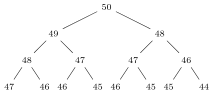
This just shows the first few levels. We see that the number of computations doubles at each step so that by the 25th level, we are doing 225= 33,554,432 calls to the function. By contrast, the iterative code runs a loop from 0 to 47, does three quick operations per iteration and is done almost instantly. The recursive method runs in O(2n) time, while the iterative method runs in O(n) time.
However, there are more efficient ways to recursively find Fibonacci numbers. One way, called memoization, involves saving the values of F49, F48, etc. as they are computed and using instead of recomputing things.
Here is another way to recursively find Fibonacci numbers. It is essentially a direct translation of the iterative code.
public static long fib(int n)
{
    if (n==1 || n==2)
        return 1;
    return helperFib(n, 0, 1, 1);
}

private static long helperFib(int n, int i, long c, long p)
{
    if (i==n-2)
        return c;
    return helperFib(n, i+1, c+p, c);
}
We have a helper function here because our recursive method has a lot of parameters that the caller shouldn't be bothered with. The fib function just handles the simple cases that n equals 1 or 2 and then sets the helperFib function in motion by essentially “initializing” the variable i to 0, and c and p to 1.
Notice how the variables in the recursive code (including the loop variable i) become parameters to the function. Also, notice how the for loop in the iterative code runs until i equals n-2, which is the base case of the helperFib function.
Let's compare the iterative code's for loop with the recursive call to helperFib.
for (int i=0; i<n-2; i++)        return helperFib(n, i+1, c+p, c);
{
    long hold = c;
    c = p+c;
    p = hold;
}
Notice that the recursive function calls itself with the i parameter set to i+1, the c parameter set to c+p and the p parameter set to c. This is the equivalent of what happens in the iterative code's for loop, where we do i++, c=c+p, and p=hold, where hold holds the old value of c.
In general, it is possible to translate iterative code to recursive code in a way similar to what we did here, where variables in the iterative code become function parameters in the recursive code.
The Sierpinski triangle
The Sierpinski triangle is a fractal object formed as follows: Start with an equilateral triangle and cut out a triangle from the middle such that it creates three equal triangles like in first part of the figure below. Then for each of those three triangles do the same thing. This gives the top middle object in the figure below. Then for each of the nine (upright) triangles created from the previous step, do the same thing. Keep repeating this process.
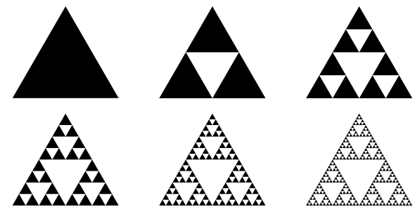
The same procedure that we apply at the start is repeatedly applied to all the smaller triangles. This makes it a candidate for recursion. Here is a program to draw an approximation to the Sierpinski triangle:
import javax.swing.*;
import java.awt.*;

public class Sierpinski extends JFrame
{
    private Container contents;
    private MyCanvas canvas;
    private int numIterations;

    public Sierpinski(int numIterations)
    {
        super("Sierpinski Triangle");
        contents = getContentPane();
        contents.setLayout(new BorderLayout());
        canvas = new MyCanvas();
        contents.add(canvas, BorderLayout.CENTER);
        setSize(450, 450);
        setVisible(true);
        setDefaultCloseOperation(JFrame.EXIT_ON_CLOSE);
        this.numIterations = numIterations;
    }

    class MyCanvas extends JPanel
    {
        public void paint(Graphics g)
        {
             sierpinski(g,200,0,0,400,400,400,numIterations);
        }

        public void drawTriangle(Graphics g, int x1, int y1, int x2,
                                 int y2, int x3, int y3)
        {
            g.drawLine(x1,y1,x2,y2);
            g.drawLine(x2,y2,x3,y3);
            g.drawLine(x3,y3,x1,y1);
        }

        public void sierpinski(Graphics g, int x1, int y1, int x2, int y2,
                               int x3, int y3, int depth)
        {
            if (depth>0)
            {
                 sierpinski(g,x1,y1,(x1+x2)/2,(y1+y2)/2,(x1+x3)/2,(y1+y3)/2,depth-1);
                 sierpinski(g,x2,y2,(x2+x3)/2,(y2+y3)/2,(x2+x1)/2,(y2+y1)/2,depth-1);
                 sierpinski(g,x3,y3,(x3+x1)/2,(y3+y1)/2,(x3+x2)/2,(y3+y2)/2,depth-1);
            }
            else
                 drawTriangle(g,x1,y1,x2,y2,x3,y3);
        }
    }

    public static void main(String[] args)
    {
        new Sierpinski(6);
    }
}
Here is the recursive part of the code:
public void sierpinski(Graphics g, int x1, int y1, int x2, int y2,
                       int x3, int y3, int depth)
{
    if (depth>0)
    {
         sierpinski(g,x1,y1,(x1+x2)/2,(y1+y2)/2,(x1+x3)/2,(y1+y3)/2,depth-1);
         sierpinski(g,x2,y2,(x2+x3)/2,(y2+y3)/2,(x2+x1)/2,(y2+y1)/2,depth-1);
         sierpinski(g,x3,y3,(x3+x1)/2,(y3+y1)/2,(x3+x2)/2,(y3+y2)/2,depth-1);
    }
    else
        drawTriangle(g,x1,y1,x2,y2,x3,y3);
}
The key to writing the code is just to worry about one case, namely the first one. When we cut out the middle triangle, we create three new triangles, whose coordinates are shown in the figure below. We then want to perform the Sierpinski triangle process on each of them, so we call sierpinski on each triangle. When we make the call, we pass the coordinates of the three vertices of the triangle (the midpoint formula is used to get them). We also have a depth variable that keeps track of how many iterations of the process we've got left. Each time we call sierpinski, we decrease that depth by 1 until we get to the base case of depth 0, which is when we actually draw the triangles to the screen.
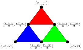
The Sierpinski triangle is one example of a fractal, an endlessly self-similar figure. Recursive fractal processes like this are used to draw realistic landscapes in video games and movies. To see some of the amazing things people do with fractals, try a web search for fractal landscapes.
Towers of Hanoi
The Towers of Hanoi is a classic problem. There are three pegs, and the one on the left has several rings of varying sizes on it. The goal is to move all the rings from that peg to the peg on the right. Only one ring may be moved at a time, and a larger ring can never be placed on a smaller ring. See the figure below.
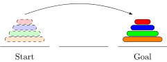
At this point, it would be good to stop reading and get out four objects of varying sizes and try the problem. Rings and pegs are not needed—any four objects of different sizes will do. The minimum number of moves needed is 15. It's also worth trying with just three objects. In that case, the minimum number of moves is 7.
We will solve the problem using recursion. The key idea is that the solution to the problem builds on the solution with one ring less. To start, here is the optimal solution with two rings:
 |
 |
 |
 |
The two-ring solution takes three moves and is pretty obvious. Shown below is the optimal seven-move solution with three rings.
 |
 |
 |
 |
 |
 |
 |
 |
Looking carefully, we can see that the solution for two rings is used to solve the three-ring problem. Steps 1, 2, and 3 are the two-ring solution for moving two rings from the left to the center. Steps 5, 6, and 7 are the two-ring solution for moving two rings from the center to the right. And overall, the three-ring solution itself is structured like the two-ring solution. Now here's the solution for four rings:
 |
 |
 |
 |
 |
 |
 |
 |
 |
 |
 |
 |
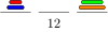 |
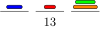 |
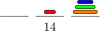 |
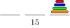 |
The general solution is a similar combination of the n-1 solution and the two-ring solution. We use the n-1 solution to move the top n-1 rings to the center, then move the bottom ring to the right, and finally use the n-1 solution to move the top three rings to the right.
It's not too hard to count the number of moves needed in general. The solution for two rings requires 3 moves. The solution for three rings requires two applications of the two-ring solution plus one more move, for a total of 2 · 3 + 1=7 moves. Similarly, the solution for four rings requires two applications of the three-ring solution plus one additional move, for 2 · 7+1=15 moves. In general, if hn is the number of moves in the optimal solution with n rings, then we have hn=2hn-1+1. And in general, hn=2n-1 moves.
This is exponential growth. Already, the solution for 10 pegs requires 210-1=1023 moves. This is a lot, but doable by hand in under an hour. The solution for 20 pegs requires over a million moves, and the solution for 30 pegs requires over a billion moves. The solution for 100 pegs requires roughly 1030 moves, which just might be able to be completed if every computer in existence worked round the clock for millions of years on the problem.
Here is a program that returns the optimal solution to the Towers of Hanoi problem.
import java.util.ArrayDeque;
import java.util.Deque;

public class Hanoi
{
    private Deque<Integer> s1, s2, s3;

    public Hanoi(int n)
    {
        s1 = new ArrayDeque<Integer>();
        s2 = new ArrayDeque<Integer>();
        s3 = new ArrayDeque<Integer>();

        for (int i=n; i>=1; i--)
            s1.push(i);

        System.out.println(s1 + " " + s2 + " " + s3);
        recursiveHanoi(s1,s3,s2,n);
    }

    public void recursiveHanoi(Deque<Integer> start, Deque<Integer> end,
                               Deque<Integer> other, int size)
    {
        if (size==1)
        {
            end.push(start.pop());
            System.out.println(s1 + " " + s2 + " " + s3);
        }
        else
        {
            recursiveHanoi(start, other, end, size-1);
            recursiveHanoi(start, end, other, 1);
            recursiveHanoi(other, end, start, size-1);
        }
    }

    public static void main(String[] args)
    {
        new Hanoi(3);
    }
}
Here is the output for the three-ring solution:
[1, 2, 3] [] []
[2, 3] [] [1]
[3] [2] [1]
[3] [1, 2] []
[] [1, 2] [3]
[1] [2] [3]
[1] [] [2, 3]
[] [] [1, 2, 3]
The code uses three stacks to represent the pegs. The class's constructor initializes the stacks and fills the left stack. All of the work is done by the recursiveHanoi method. The method takes three stacks—start, end, and other— as parameters, as well as an integer size. Any move can be thought of as moving size number of rings from start to end, using other as a helper peg.
The base case of the recursion is size=1, which is when we are moving a single ring from one peg to another. We accomplish that by popping the “peg” from the start stack and pushing it onto the end stack. At this point we also print out that stacks, so that every time a switch is made, the stacks are printed.
The recursive part of the method moves size-1 rings from the start stack to the helper stack (other), then moves the bottom ring from the start stack to the end stack, and finally moves size-1 rings from the helper stack to the end stack.
Summary
Sometimes recursion almost seems like magic. All you have to do is specify how to use the solution to the smaller problem to solve the larger one, take it on faith that the smaller one works, and you're essentially done (once you do the base case, which is often simple).
For example, here again is recursive solution to reversing a string: break off the first character, reverse the remaining characters and add the first character to the end. The code for this is:
return reverse(s.substring(1)) + s.charAt(0);
We just assume that reverse correctly reverses the smaller substring and then add the first character to the end. This, plus the base case to stop the recursion, are all that we need.
In Java, a simple rule for when to use recursion might be to use it when it gives a simpler, easier-to-code solution than an iterative approach and doesn't risk a stack overflow error or other inefficiency (like with the first Fibonacci function we did). A good example of an appropriate use of recursion is for calculating permutations. Iterative code to generate permutations is somewhat more complicated than the recursive code. And there is no risk of a stack overflow as we couldn't generate permutations for very large values of n recursively (or iteratively) because there are so many permutations (n! of them).
The take-home lesson is that in Java, most code is done iteratively, and recursion is useful on occasion.
Exercises
- Rewrite the reverse function from the introductory recursion section so that it works by trimming off the last character instead of the first character.
- Write recursive implementations of the following. In many cases an iterative solution would be much easier, but this exercise is for practice thinking recursively. Assume that any lists in this problem are lists of integers.
-
contains(s, c)— returns whether the stringscontains the characterc -
indexOf(s, c)— returns the index of the first occurrence of the charactercin the stringsand -1 ifcis not ins. -
count(s,c)— returns a how many times the charactercoccurs in the strings -
repeat(s, n)— returns a string consisting ofncopies of the strings -
toUpperCase(s)— returns a string with all the lowercase letters ofschanged to uppercase. -
swapCases(s)— returns a string with all the lowercase letters ofschanged to uppercase and all the uppercase letters ofschanged to lowercase. -
alternateSum(list)— returns the alternating sum of the list. For example, for[1,2,3,4,5], the method should return 1-2+3-4+5, which is 3. -
removeAll(s,c)— returns the string obtained by removing all occurrences of the charactercfrom the strings -
range(i,j)— returns a list containing the integers fromithroughj-1 -
stringRange(c1,c2)— returns a string containing the characters alphabetically fromc1toc2, not includingc2. For instance,stringRange('b','f')should return"bcde". -
containsNoZeroes(list)— returns true if there are no zeroes in the list and false otherwise. -
digitalRoot(n)— returns the digital root of the positive integer n. The digital root of n is obtained as follows: Add up the digits n to get a new number. Add up the digits of that to get another new number. Keep doing this until you get a number that has only one digit. That number is the digital root. -
max(list)— returns the maximum element oflist -
firstDiff(s, t)— returns the first index in which the stringssandtdiffer. For instance, ifs="abc"andt="abd", then the function should return 2. Ifs="ab"andt="abcde", the function should also return 2. -
matches(s, t)— returns the number of indices in which the stringssandtmatch, that is the number of indices i for which the characters ofsandtat index i are exactly the same. -
oneAway(s, t)— returns true if stringssandtare the same length and differ in exactly one character, likedrawanddraborwaterandwafer. -
isSorted(list)— returns whether the elements oflistare in increasing order -
equals(list,list2)— returns whetherlist1andlist2are equal -
evenList(list)— returns whether thelisthas an even number of elements. Do this without actually counting how many elements are in the list. -
sameElements(list1,list2)— returns whetherlist1andlist2have the same elements with the same frequencies, though possibly in different orders. For instance, the function would return true[1,1,2,3]and[2,1,3,1]but false for[1,1,2,1]and[2,2,1,2]. -
countStart(list)— counts the number of repeated elements at the start oflist -
removeStart(list)— removes any repeated elements from the start oflist -
duplicate(list,n)— duplicates every item inlistntimes. For instance, witha=[1,2,2,3]andn=3, the method would return[1,1,1,2,2,2,2,2,2,3,3,3]. -
triple(s)— returns a string with each character ofsreplaced by three adjacent copies of itself. For instance,triple("abc")should return"aaabbbccc". -
sumElementsAtEvenIndices(list)— returns the sum of the elements at indices 0, 2, 4, …. For instance, iflistis[1,4,7,10,13,16], this method would return 21 (which is 1+7+13). -
addOneToEverything(list)— returns a new list with 1 to every element of the original. For instance, iflistis[1,4,7,10]then this method would return the list[2,5,8,11].
-
- Write recursive implementations of the following. In many cases an iterative solution would be much easier, but this exercise is for practice thinking recursively. Assume that any lists in this problem are lists of integers.
-
hasAnEvenNumberOf(s, c)— returns true if the stringshas an even number of occurrences of the charactercand false otherwise. Remember that 0 is an even number. -
allEven(list)— returns true if all the elements oflistare even. (Assumelistis a Java list of integers.) -
stringOfSquares(n)— returns a string containing all the perfect squares from 12 through n2, separated by spaces. For instance,stringOfSquares(5)should return the string"1 4 9 16 25". -
containsNegativePair(list)— returnstrueif anywhere in the list there are consecutive integers that are negatives of each other. It returnsfalseotherwise. For instance, it would return true for the list[2,3,5,-5,6,-9]because that list contains the consecutive pair, 5, -5, which are negatives of each other. -
swap(s)— assumingsis a string consisting of zeros and ones, this method returns a string with all of the ones changed to zeros and all of the zeros changed to ones. For instance,swap("00001101")should return"11110010". -
gcd(m,n)— returns the greatest common divisor of m and n -
factorial(n)— returns n!, where n! is the product of all the integers between 1 and n. For example, 5!=5 · 4 · 3 · 2 · 1 = 120. -
flatten(list)— returns a flattened version of thelist. What this means is that iflistis a list of lists (and maybe the lists are nested even deeper), then the result will be just a flat list of all the individual elements. For example,[1,2,3,4,5,6,7,8,9,10]is the flattened version of[1,[2,3],[4,5],[6,[7,8,[9,10]]]]. -
compress(list)— compresses the listaso that all duplicates are reduced to a single copy. For instance,[1,2,2,3,4,4,4,4,5,5,6]gets reduced to[1,2,3,4,5,6]. -
runLengthEncode(list)— performs run-length encoding on a list. Given a list it should return a list consisting of all lists of the form[x,n], wherexis an element the list andnis its frequency. For example, the encoding of[a,a,b,b,b,b,c,c,c,d]is[[2,a],[4,b],[3,c],[1,d]]. -
expand(s)— given a string where the characters at even indices are letters and the characters at odd indices are single digits (like"a3b8z3e0y2"), this method returns the string obtained by replacing each character at an even index with a number of copies of it equal to the digit immediately following it. For the string given above, the result should be"aaabbbbbbbbzzzyy". -
superRepeat(list, n)— takes a list calledlistand an integernand returns a new list which consists of each element oflistrepeatedntimes, in the same order as inlist. For example, iflist=[6,7,8,8,9]and we callsuperRepeat(list, 4), the method should return the list[6,6,6,6,7,7,7,7,8,8,8,8,8,8,8,8,9,9,9,9]. -
partitions(n)— returns a list of all the partitions of the integern. A partition of n is a breakdown of n into positive integers less than or equal to n that sum to n, where order doesn't matter. For instance, all the partitions of 5 are 5, 4+1, 3+2, 3+1+1, 2+2+1, 2+1+1+1, and 1+1+1+1+1. Each partition should be represented as a string, like"2+1+1".
-
- Rewrite the sum function from this section so that it uses a parameter to the function called
totalto keep a running total. - Translate the following code into recursive code using the technique outlined in this section.
-
public static List<Integer> f(int n) { List<Integer> a = new ArrayList<Integer>() for (int i=2; i<n; i++) { if (i*i%5==1) a.add(i) } } -
public int f(int n)
{
    for (int i=0; i<n; i++)
    {
        for (int j=i; j<n; j++)
        {
            for (int k=j; k<n; k++)
            {
                if (i*i+j*j=k*k)
                    count++;
            }
        }
    }
    return count;
}
-
- What does the following recursive method do?
public static boolean f(String s) { if (s.length()==0 || s.length()==1) return true; if (s.charAt(0)!=s.charAt(s.length()-1)) return false; return f(s.substring(1,s.length()-1)); } - Rewrite the binary search algorithm from this section recursively.
- Rewrite the permutations function from this section to return a list of the permutations of an arbitrary string. For instance, when called on
"abc", it should return[cba, bca, bac, cab, acb, abc]. - Rewrite the permutations function from this section so that it returns lists of integer lists instead of strings. For instance, when called with n=2, it should return
[[1,2], [2,1]]. - Rewrite the permutations function from this section iteratively.
- Rewrite the combinations function from this section iteratively.
- Write a recursive function called
combinationsWithReplacement(n,k)that returns all the k-element combinations with replacement of the set {1,2,…,n} as a list of strings, like the combinations function from this section. Combinations with replacement are like combinations, but repeats are allowed. For instance, the two-element combinations with replacement of {1,2,3,4} (shorthand 1234) are 11, 12, 13, 14, 22, 23, 24, 33, 34, and 44. - Increasing sequences — Write a recursive function that takes an integer n and returns a list consisting of all strings of integers that start with 1, end with n, and are strictly increasing.
Here is how to solve the problem. These are the solutions for n=1 through 5:
n=1: 1
n=2: 12
n=3: 13, 123
n=4: 14, 124, 134, 1234
n=5: 15, 125, 135, 145, 1235, 1245, 1345, 12345Looking at how we get the strings for n=5, they come from each of the strings for n=1 2, 3, and 4, with a 5 added to the end. This works in general: to get all the increasing strings ending with n, take all the increasing strings that end with 1, 2, …, n-1 and add n to the end of each of them.
- Modify the program from this section to recursively generate approximations to the Sierpinski carpet. The first few approximations are shown below.
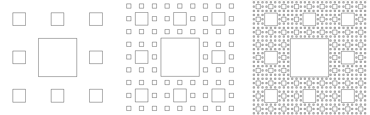
Binary Trees
Tree structures are fairly common in everyday life. For example, shown below on the left is tree of the outcomes of flipping a coin three times. On the right is a simplified version of part of a phylogenetic tree, one that shows the family relationships of animal species.
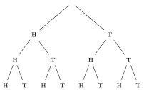 |
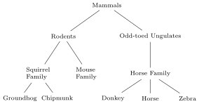 |
These are just two simple examples. Trees are especially important in computer science. Of particular interest are binary trees, trees where each node has no more than two children.
First, a little terminology. Consider the tree below.
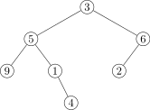
The circles are called nodes. Each node has a data value associated to it. The node at the top of the tree is called the root. Each node has up to two children, which we will refer to as its left child and right child. The nodes at the end of the tree are called leaves.
Implementing a binary tree
Our implementation will be similar to our linked list implementation. Each node of the tree will be represented as a Node object. The Node class will have three fields: a field to hold the node's data, a link to the left child, and a link to the right child. Here is the start of the BinaryTree class:
public class BinaryTree<T>
{
    private class Node
    {
        public T data;
        public Node left
        public Node right;

        public Node(T data, Node left, Node right)
        {
            this.data = data;
            this.left = left;
            this.right = right;
        }
    }

    private Node root;

    public BinaryTree()
    {
        root = null;
    }
}
The BinaryTree class has a class variable, root, to represent the root of the tree. This is analogous to our linked list implementation, which had a class variable, front, representing the front node of the list. The constructor creates an empty tree by setting the root to null.
Adding things to the tree
Next, we have a method add that adds a new node to the tree. We need to be able to specify where to add the node. One way is to specify the node's parent. We will take another approach, where we specify the location with a string of L's and R's that describe the path we take to get to the added node. For instance, the node to be added in the figure below is specified by LRL.
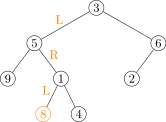
Here is the add method:
public void add(T data, String location)
{
    if (location.equals(""))
    {
        root = new Node(data, null, null);
        return;
    }

    String parentPart = location.substring(0,location.length()-1);
    char childPart = location.charAt(location.length()-1);

    Node n = root;
    for (char c : parentPart.toCharArray())
        n = c=='L' ? n.left : n.right;

    if (childPart=='L')
        n.left = new Node(data, null, null);
    else
        n.right = new Node(data, null, null);
}
The first part of the add function considers the case where the location is the empty string. Remember that our string consists of L's and R's. A string that has none of those means we don't go anywhere. In other words, we stay at the root.
Otherwise, we break the location string into two pieces: all the characters but the last, and the last character. That last character represents whether the new node will be the left or the right child of its parent. The rest of the string represents the route we take to get to the parent. That's what the loop is used for. We loop through the location string, moving left if we encounter an L and right otherwise. Note that the code uses Java's ternary operator, which essentially acts like an if/then/else compressed into a single line.
When the for loop ends, we are at the parent of the new node. The remainder of the function uses the last character of the location string to determine whether the new node is the left or right child of the parent and then it creates the new node.
One thing to consider here is what happens if the user passes the method an invalid string, like one that contains letters other than L and R. Our code does not handle that case. A good thing to do would be to raise an illegal argument exception.
Deleting from the tree
Our method will be called prune because it is like pruning a branch from a real-life tree. Not only is the node removed, but the entire subtree starting at that node is removed. See the figure below.
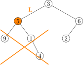
We use a string to specify the location to be pruned, just like we did with the add method. The first case to consider is if we are deleting the root. This can be accomplished by simply setting root to null. Otherwise, we loop through the location string, just like with the add method, moving left or right down the tree as we encounter L's and R's. We then sever either the parent's left link or its right link to the child. We do this by setting it to null, which will effectively remove that whole branch from the tree.
public void prune(String location)
{
    if (location.equals(""))
    {
        root = null;
        return;
    }

    Node n = root;
    String parentPart = location.substring(0,location.length()-1);
    char childPart = location.charAt(location.length()-1);

    for (char c : parentPart.toCharArray())
         n = (c=='L') ? n.left : n.right;

    if (childPart == 'L')
        parent.left = null;
    else
        parent.right = null;
}
Printing the contents of the tree
Let's now add a toString method for printing the tree. There are a number of different ways we can print the contents of the tree. What we'll do here is print out an in-order traversal of the tree. The way that works is we always visit nodes in the order left-center-right. That is, from any given node, we will always print out everything in the left subtree, then the node's own value, and finally everything in its right subtree. This is a recursive process. From a given node we first print out the in-order traversal of the left subtree, then the value of the node, then the in-order traversal of the right subtree. Let's look at how this works on the tree below:

Start at the root. According the in-order rule, we first look at its left subtree. So we're now at the node labeled with 5. Again, recursively following the rule, we look at this node's left subtree. We're now at the node labeled 9. Its left subtree is empty, so following the in-order rule, we then look at the node itself, which has data value 9, and that's the first thing that gets printed. The node labeled 9 has no right subtree, so we back up to the previous node. Having finished its left subtree, we visit the node itself, and print out a 5. We then visit its right subtree and apply the same process. In the end, we get 9 5 1 4 3 6 2.
As the process described is recursive, we will use recursion here. The toString method is shown below:
@Override
public String toString()
{
    return toStringHelper(root);
}

private String toStringHelper(Node n)
{
    if (n == null)
        return "";
    return toStringHelper(n.left)+ n.data + " " + toStringHelper(n.right);
}
Notice that the toString method needs a helper method. The recursion requires us to add a parameter to the method to keep track of where we are in the tree. However, the toString method (as per Java's definition of it) should have no parameters. So we create a separate method that has a parameter and does all the work, and we call that method from toString. The toString method just gets the recursion started by feeding toStringHelper a starting node, the tree's root.
We make the helper method a private method because it is not something users of our class need to see. It is just something our class needs to get some work done internally.
The toStringHelper method has a base case, which is a null node. In that case, there is no data value to print, so it returns the empty string. For the recursive part, we follow the prescription left-center-right. All we do here is tell how to combine the results from the left, center, and right subtrees, and let recursion take care of the rest.
Here is an alternate toStringHelper method that prints out the path to each node as a string of L's and R's. To get the path, we add a parameter location to the helper function. In the recursion, we add an "L" or "R" to the previous location depending on whether we are moving on to the left or right subtree.
private String toStringHelper(Node n, String location)
{
    if (n == null)
        return "";

    if (n == root)
        return toStringHelper(n.left, location+"L") + " " + "root: " + n.data +
               "\n" + toStringHelper(n.right, location+"R");

    return toStringHelper(n.left, location+"L") + " " + location + ": " +
           n.data + "\n" + toStringHelper(n.right, location+"R");
}
For the tree shown earlier in this section, here is the output of this toString method:
LL: 9
L: 5
LR: 1
LRR: 4
root: 3
RL: 2
R: 6
There are two other similar ways of traversing trees: pre-order and post-order. For pre-order, we go center-left-right, and for post-order, we go left-right-center. Two different traversals of a tree—breadth-first and depth-first—are the subjects of part of Exercise , as well as Section .
The size of a tree
The recursive approach we took to traversing the tree sets the pattern for most binary tree methods. For example, here is a method that returns the number of nodes in the tree:
public int size()
{
    return sizeHelper(root);
}

private int sizeHelper(Node n)
{
    if (n == null)
        return 0;
    return 1 + sizeHelper(n.left) + sizeHelper(n.right);
}
We have a public/private pair. The public method size is the one that the user sees. It acts as a wrapper around the private method recursiveSize that does all the work. Again, the reason for two methods is that the recursive algorithm we use requires the method to have a parameter keeping track of where we are in the tree. To get the size of the tree, the user should just have to use tree.size(), not tree.size(tree.root).
The way the recursive method works is to break the tree down into smaller subtrees, namely the left subtree and the right subtree from each node. The number of elements in the part of the tree including the current node and all its descendants is equal to the size of the left subtree plus the size of the right subtree plus 1 (for the current node). The base case of the recursion is a null node, which contributes nothing to the size of the tree. Thus we return 0 in that case. Here is an example of how a tree is broken down:
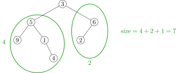
The key to writing a method like this is to think about how to combine the size of the left subtree and the right subtree to get the answer for the entire tree. In the example above, we see that the size of the tree is 4+2+1, which is the size of the left subtree plus the size of the right subtree plus 1 for the node itself.
The number of leaves on the tree
Here is another example to get a feel for how recursion is useful on binary trees. The method below returns a count of how many leaves the tree has.
public int leafCount()
{
    return leafCountHelper(root);
}

private int leafCountHelper(Node n)
{
    if (n == null)
        return 0;
    if (n.left == null && n.right == null)
        return 1;
    return leafCountHelper(n.left) + leafCountHelper(n.right);
}
The recursive process we use here is similar to the size method in that the number of leaves is the sum of the leaves in the left subtree and the right subtree. Notice that we don't add an additional 1 here, like we did in the size method, because the current node is not necessarily a leaf itself. See the figure below:
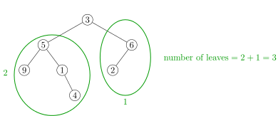
Notice also that we have two base cases, one for if we've reached a null node and one for if we've found a leaf. To check to see if a node is a leaf, we just have to check to see if both of its children are null.
The height of a tree
Let's look at a method that returns the height of a tree, which is how many levels deep the tree goes. Formally, an element is said to be at level k of the tree if we have to follow k links to get to it from the root. The root is at level 0, the root's two children are at level 1, their children are at level 2, etc. Here is the code for the method:
public int height()
{
    return heightHelper(root);
}

private int heightHelper(Node n)
{
    if (n == null)
        return 0;
    return 1 + Math.max(heightHelper(n.left), heightHelper(n.right));
}
The key is to imagine how to determine the height of a tree if all we know is the height of its left and right subtrees. To do this, we have to notice that the height of a tree is equal to 1 more than the height of either its left or the right subtree, whichever is larger. This is what the last line of the helper function does. See the figure below.
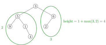
This is how to think recursively—figure out how the problem can be solved in terms of smaller versions of itself. You don't actually have to specify how to move through the tree. Instead specify how to combine the solutions to the subproblems to get a solution to the whole, and specify some base cases to stop the recursion.
The exercises ask you to write a number of other methods for the binary tree class. Many of them follow this pattern, consisting of a public/private pair, and a recursive algorithm that combines the results from the left and right subtrees of each node.
A contains method
We'll try one more method, a contains method that tells if the tree contains a certain value. Again, we approach this by trying to figure out how we take the answers for the left and right subtrees and combine them to get the answer for the whole tree. Here is the code:
public boolean contains(T x)
{
    return containsHelper(root, x);
}

private boolean containsHelper(Node n, T x)
{
    if (n == null)
        return false;
    if (n.data.equals(x))
        return true;
    return containsHelper(n.left, x) || containsHelper(n.right, x);
}
The way it works is we basically return true if the current node's data equals the data we're looking for or if the value is in either the node's left or the right subtree. The last line of the helper checks the left and right subtrees. If either of them contains the value, then the entire OR expression will be true and otherwise it will be false. See the figure below.
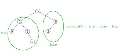
The entire binary tree class
Here is the entire class:
public class BinaryTree<T>
{
    private class Node
    {
        public T data;
        public Node left;
        public Node right;

        public Node(T data, Node left, Node right)
        {
            this.data = data;
            this.left = left;
            this.right = right;
        }
    }

    public Node root;

    public BinaryTree()
    {
        root = null;
    }

    public void add(T data, String location)
    {
        if (location.equals(""))
        {
            root = new Node(data, null, null);
            return;
        }

        String parentPart = location.substring(0,location.length()-1);
        char childPart = location.charAt(location.length()-1);

        Node n = root;
        for (char c : parentPart.toCharArray())
            n = c=='L' ? n.left : n.right;

        if (childPart=='L')
            n.left = new Node(data, null, null);
        else
            n.right = new Node(data, null, null);
    }

    public void prune(String location)
    {
        if (location.equals(""))
        {
            root = null;
            return;
        }

        Node n = root;
        String parentPart = location.substring(0,location.length()-1);
        char childPart = location.charAt(location.length()-1);

        for (char c : parentPart.toCharArray())
            n = (c=='L') ? n.left : n.right;

        if (childPart == 'L')
            parent.left = null;
        else
            parent.right = null;
    }

    @Override
    public String toString()
    {
        return toStringHelper(root, "");
    }

    private String toStringHelper(Node n, String location)
    {
        // in-order traversal
        if (n == null)
            return "";

        if (n == root)
            return toStringHelper(n.left, location+"L") + " " + "root: " + n.data +
            "\n" + toStringHelper(n.right, location+"R");

        return toStringHelper(n.left, location+"L") + " " + location + ": " +
               n.data + "\n" + toStringHelper(n.right, location+"R");
    }


    /* The following simpler toStringHelper that just prints out the elements of
       the tree using an in-order traversal without labeling where they are from. */

    private String toStringHelper(Node n)
    {
        // in-order traversal
        if (n == null)
            return "";
        return toStringHelper(n.left) + " " + n.data + " " +
               toStringHelper(n.right);
    }

    public boolean isEmpty()
    {
        return root==null;
    }

    public int size()
    {
        return sizeHelper(root);
    }

    private int sizeHelper(Node n)
    {
        if (n == null)
            return 0;
        return 1 + sizeHelper(n.left) + sizeHelper(n.right);
    }

    public int leafCount()
    {
        return leafCountHelper(root);
    }

    private int leafCountHelper(Node n)
    {
        if (n == null)
            return 0;
        if (n.left == null && n.right == null)
            return 1;
        return leafCountHelper(n.left) + leafCountHelper(n.right);
    }

    public int height()
    {
        return heightHelper(root);
    }

    private int heightHelper(Node n)
    {
        if (n == null)
            return 0;
        return 1 + Math.max(heightHelper(n.left), heightHelper(n.right));
    }

    public boolean contains(T x)
    {
        return containsHelper(root, x);
    }

    private boolean containsHelper(Node n, T x)
    {
        if (n == null)
            return false;
        if (n.data.equals(x))
            return true;
        return containsHelper(n.left, x) || containsHelper(n.right, x);
    }
}
Summary
Exercise in this chapter is pretty important. It is about implementing some methods for this binary tree class. The trick to it is the same as what we've seen for the methods above—use recursion by thinking about an arbitrary node on the tree and thinking about how to answer the question based on the answers for its left and right subtrees.
For instance, recall the size method that returns the number of nodes in the tree. The way it works is we imagine we're at some node in the tree. We then call the size method on its left and right subtrees, and we ask how do we use those answers to get the overall size. The answer is that the size is the size of the left subtree, plus the size of the right subtree, plus 1 for the node itself. In code, it becomes this:
return 1 + sizeHelper(n.left) + sizeHelper(n.right);
Most of those exercises work in the same way, where you will combine the answers from the left and right subtrees to get the overall answer.
Running times of the methods
The add method runs in O(n) in the worst case. The worst case here is if the tree is a path, where each node, except the last, has exactly one child. If we try to add to the bottom of a tree of this form, we have to walk through all n nodes to get to the bottom of the tree. On the other hand, if the tree is more-or-less balanced, where for any given node both its left and right subtrees have roughly the same size, then adding is O(log n). This is because with each left or right turn we take to get to the desired node, we essentially are removing half of the tree from consideration. These ideas will be especially important in the next chapter.
The analysis above also applies also to the prune method. The rest of the methods all run in O(n) time because they visit each of the nodes exactly once, doing a few O(1) operations at each node.
A different approach
There is another approach we can take to implementing binary trees that is simpler to code, but less user-friendly to work with. The key observation here is to think of a tree as a recursive data structure. Each node of the tree consists of a data value and links to a left and a right subtree. And those subtrees are of course binary trees themselves. Here is how such a class might look (using integer data for simplicity):
public class Tree
{
    private int data;
    private Tree left, right;

    public Tree(int data, Tree left, Tree right)
    {
        this.data = data;
        this.left = left;
        this.right = right;
    }
}
Here a binary tree and its declaration using this class. The declaration is spread across several lines for readability.
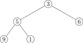
Tree tree = new Tree(3,
                     new Tree(5,
                              new Tree(9, null, null),
                              new Tree(1, null, null)),
                     new Tree(6, null, null));
We could then add methods to our class if we want. Here's a toString method:
@Override
public String toString()
{
    return toStringHelper(this);
}

public String toStringHelper(Tree tree)
{
    if (tree==null)
        return "";
    return toStringHelper(tree.left) + " " + tree.data + toStringHelper(tree.right);
}
We can see that this is very similar to the earlier toString method. In fact, the other recursive algorithms we wrote would change very little with this new approach.
To add a node to a binary tree, we specify its data value, its parent, and whether to go left or right. Here is the add method:
public void add(int data, Tree parent, char leftRight)
{
    if (leftRight=='L')
        parent.left = new Tree(data, null, null);
    else
        parent.right = new Tree(data, null, null);
}
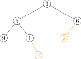
To add the nodes indicated in the tree above, we would use the following:
tree.add(2, tree.right, 'L');
tree.add(4, tree.left.right, 'R');
The prune method is quite similar:
public void prune(Tree parent, char leftRight)
{
    if (leftRight == 'L')
        parent.left = null;
    else
        parent.right = null;
}
This approach and the earlier node-based approach are actually quite similar. In the earlier approach the recursion is hidden in the Node class, which has references to itself. That earlier approach is a little more user-friendly, but that friendliness came at a cost of more work to code the methods.
Either of the two implementations of binary trees gives a good basis to work from if you need a binary tree class for something. This is important as there is no binary tree or general tree class in the Collections Framework, so if you need an explicit binary tree class, you either have to code one up yourself or look around for one.
Applications
Binary trees and more general trees are a fundamental building block of other data structures and algorithms and form a useful way to represent data. They show up in networking algorithms, compression algorithms, and databases. In this chapter we will see binary search trees and heaps, which are specialized binary trees used for maintaining data in order.
A computer's file system can be thought of as a tree with the directories and files being the nodes. The files are leaf nodes, and the directory nodes are nodes whose children are subdirectories and files in the directory.
Another place binary trees show up is in parsing expressions. An expression is broken down into its component parts and is represented using a tree like in the example below, which represents the expression 3+4*5-6.
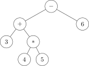
Trees also provide a natural way to structure moves from a game. For example, the potential moves in a game of tic-tac-toe can be represented with the following tree: The root node has nine children corresponding to nine possible opening moves. Each of those nodes has eight children corresponding to the eight possible places the second player can go. Each of those nodes has children representing the first player's next move. And those children have children, and so on to the end of the tree. A computer player can be implemented by simply searching through the tree looking for moves that are good according to some criterion.
Binary trees are also one of the simplest examples of graphs, covered in this chapter.
Exercises
- Add the following methods to the binary tree class of this section.
-
count(x)— returns how many things in the tree are equal tox. When checking if things are equal tox, use.equals()instead of==. -
preOrderPrintandpostOrderPrint— which are analogous toinOrderPrintexcept they use preorder and postorder traversals, respectively. -
get(location)returns the data value at the node specified by the stringlocation -
set(location, data)changes the data value at the node specified by the stringlocationto the new valuedata. -
leaves()— returns a list containing the data in all the leaves of the tree -
level(location)— returns the level of the node specified by the stringlocation, assuming the root is at level 0, its children are at level 1, their children are at level 2, etc. -
printLevel(k)— prints all of the elements at levelk -
descendants(location)— returns the number of descendants of the node specified by the stringlocation -
isUnbalanced()— returns true if there is some node for which either its left subtree or right subtree is more than one level deeper than the other -
equals(t)— returns true if the tree is equal to the treet. Two trees are considered equal if they have the same values in the exact same tree structure. -
numberOfFullNodes()— returns how many nodes in the tree have exactly two children (only children, not grandchildren or other descendants) -
parenthesizedRep()— returns a string containing a parenthesized representation of a tree. The basic structure of the representation at a nodenis (data stored inn, representation of left subtree, representation of right subtree). If a node doesn't have a left or a right subtree, the representation for the missing subtree is*. As an example, the tree below has the following representation:(3,(5,(9,*,*),(1,*,(4,*,*))),(6,(2,*,*),*))
-
breadthFirstSearch(x)— determines if the tree containsxusing a breadth-first search. Such a search starts at the root of the tree, and then examines all of the nodes at level 2, then all of the nodes at level 3, etc. -
depthFirstSearch(x)— determines if the tree contains thexusing a depth-first search. Such a search starts at the root and always follows each branch to the end before backing up.
-
- Our binary tree class works with generic types.
- Make the class less general. Write it so that it only works with integer data.
- Add to the class from part (a) a method,
min, that returns the minimum element in the tree. - Add to the class from part (a) a method
depthSumthat returns the sum of the elements in the tree, weighted by depth. The root is weighted by 1, each of its children is weighted by 2, each of their children is weighted by 3, etc. - Read ahead to this section and rewrite the original binary tree class to implement the
Comparableinterface. Then add in a methodminthat returns the minimum element in the tree.
- Rewrite the
sizemethod using an iterative, instead of recursive, algorithm. - Rewrite the binary tree class to represent a general tree where each node can have an arbitrary number of children. To do this, use a list of nodes in place of the
leftandrightvariables. - Write a binary tree class that uses an dynamic array instead of a linked structure. Use the following technique: The root is stored at index 0. Its children are stored at indices 1 and 2. The children of the root's left child are stored at indices 3 and 4, and its right children are stored at indices 5 and 6. In general, if the index of a node is i, then its left and right children are stored at indices 2i+1 and 2i+2, respectively. The class should have three methods:
-
setRoot(value)— sets the value of the root node -
set(location, value)— takes a string,location, of L's and R's representing the location, and sets the corresponding node tovalue -
toString()— returns a string representing an in-order traversal of the tree
-
- Add the methods from Exercise to the dynamic array implementation from the previous exercise.
Binary Search Trees, Heaps, and Priority Queues
This chapter is about data structures that are efficient at storing ordered data.
Binary Search Trees
Let's suppose we have a list containing some data in sorted order. The data changes from time to time as things are removed from the list and new things are added to the list, but the list needs to remain sorted at all times.
It's not to hard to write an algorithm to insert an element in the proper place in the list—just step through the list element by element until you reach an element that is larger than the one you want to insert and insert the new element there. For example, the following method will do just that:
public static void addSorted(int element, List<Integer> list)
{
    int i=0;
    while (i<list.size() &&  element>list.get(i))
        i++;
    list.add(i, element);
}
The only problem is that the worst-case and average-case running times of this algorithm are O(n) because we have to step through all n items of the list in the worst case and n/2 items on average. Moreover, inserting the new element into the list is an O(n) operation. This can add up if we have a list of millions of items that we are continually adding and deleting from.
But, by storing our data in a more clever way, in something called a binary search tree (BST), we can get the running time down to O(log n). It is worth noting once more how big a difference there is between n and log n: if n=1,000,000, then log n ≈ 20. There is a huge difference between a program that takes 1,000,000 milliseconds to run and a program that takes 20 milliseconds to run.
Recall from this section that the binary search algorithm is an O(log n) algorithm for finding an element in a list. It works by breaking continually breaking the data into halves and essentially throwing away the half that doesn't contain the value we are looking for. It is similar to how we might look through a long list for a value—look at an entry somewhere in the middle. Assuming we didn't find it on the first try, if the entry is bigger than the one we want we know not to bother with the upper half of the list and to just look at the lower half of the list, and if the entry is smaller than the one we want, we can just focus on the upper half of the list. We then apply the same procedure to the appropriate half of the list and keep doing so, cutting the search space in half at each step until we find the value we want. This continuous cutting in half is characteristic of logarithmic algorithms.
A BST can be thought of as combination of a binary tree and the binary search algorithm. Formally, a BST is a binary tree with one special property:
For any given node N, each element in its left subtree is less than or equal to the value stored in N and each element in its right subtree is greater than the value stored in N.
To add an element to a BST we start at the root and traverse the tree comparing the value to be added to the value stored in the current node. If the value to be added is less than or equal to the value in the current node, we move left; otherwise, we move right. We continue this until we reach the end of the tree (reach a null link).
For example, suppose we add the integers 5, 11, 19, 6, 2, 4, 2, 3, 26 to the BST in exactly that order. The figure below shows the evolution of the tree.
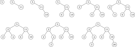
Try this on paper for yourself to get a good sense of how the BST property works.
It might not be obvious that the data stored in this tree is actually sorted, but it is. The key is to do an in-order traversal of the tree. Remember that an in-order traversal visits nodes in the order left-middle-right, visiting the entire left subtree, then the node itself, then the right subtree. The BST property guarantees that the data values of everything to the left of a node will be less than or equal its value and everything to the right will be greater, which means that an in-order traversal will return the data in exactly sorted order.
Implementing a BST
As a BST is a binary tree, we will use a lot of the code from our binary tree class. In particular, we will use a very similar node class and the same toString method that uses an in-order traversal. In fact, by printing out our BST, we see where “in-order traversal” gets its name: the values will be printed in order.
One change we will make for now is to just make our class work with integers. The reason for this is we have to compare values, and not all data types can be compared. A little later in the chapter we will see how to make it work for more general types. Here is the start of the class:
public class BinarySearchTree
{
    private class Node
    {
        int data;
        Node left, right;

        public Node(int data, Node left, Node right)
        {
            this.data = data;
            this.left = left;
            this.right = right;
        }
    }

    private Node root;

    public BinarySearchTree()
    {
        root = null;
    }

    @Override
    public String toString()
    {
        return toStringHelper(root);
    }

    private String toStringHelper(Node n)
    {
        // in-order traversal
        if (n==null)
            return "";
        return toStringHelper(n.left) + " " + n.data + " " + toStringHelper(n.right);
    }
}
Adding things to a BST
The idea behind adding things to a BST is simply to follow the BST property node by node. Start at the root and compare the value to be added with the root's value. If the value is less than or equal to the root's value, then go left and otherwise go right. Then do the same thing at the new node, moving left or right by comparing data values. We continue this until we read the end of the tree and add the new node there.
For instance, in the example below, let's suppose we are adding a 7 into the BST.
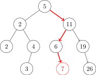
We start by comparing 7 to the root's value 5. Since 7>5, we move right. Then we compare 7 to the next node's value, 11, and since 7≤ 11, we move left. Then comparing 7 to 6, we see 7>6 so we move right. At this point we stop and add the new node because the moving right leads to a null node.
To code this, we first need a special case if the root is null. With that out of the way, we run a loop to move through the tree. At each stage, we compare the value being added with the current node's value. At each step there are four possibilities: move left, move right, add the new node at the left link of the current node, or add the new node at the right. The latter two possibilities are used when we reach the end of the tree. This is coded below:
public void add(int data)
{
    if (root == null)
    {
        root = new Node(data, null, null);
        return;
    }

    Node n = root;
    while (true)
    {
        if (data <= n.data && n.left == null)
        {
            n.left = new Node(data, null, null);
            return;
        }

        else if (data <= n.data)
            n = n.left;

        else if (data > n.data && n.right == null)
        {
            n.right = new Node(data, null, null);
            return;
        }

        else
            n = n.right;
    }
}
Here is some code to test the add method:
BinarySearchTree bst = new BinarySearchTree();
List<Integer> list = new ArrayList<Integer>();
Collections.addall(list, 5, 11, 19, 6, 2, 4, 2, 3, 26);
for (int x : list)
    bst.add(x);
System.out.println(bst);
2 2 3 4 5 6 11 19 26
Notice that the data is displayed in sorted order.
A contains method
For a little more practice, here is a contains method that tests if a BST contains a value or not:
public boolean contains(int data)
{
    Node n = root;
    while (n != null)
    {
        if (data == n.data)
            return true;
        else if (data <= n.data)
            n = n.left;
        else
            n = n.right;
    }
    return false;
}
The code is similar to the add method. We use a while loop to visit the nodes. If the data value is less than the current node's data value, then move left down the tree, if it is greater, move right, and if it's equal return true. If we reach a null node, then we've fallen off the end of the tree and we know the value is not there, so we return false.
Removing values
Removing a data value from a BST is a little tricky as we can't just delete its corresponding node from the tree as that would cut off its descendants as well, essentially removing their data values from the tree. We will break the problem into three separate cases. All of them require that we first locate the node to be deleted and its parent. Here is the code to do that:
Node n = root, parent = null;
while (data != n.data)
{
    parent = n;
    n = (data > n.data) ? n.right : n.left;
}
This very similar to the code we used for the add method. The difference is we also maintain a variable called parent that will end up being the parent of the node to be deleted.
Now that we've found the node, here are the cases for deleting it.
Case 1: Deleting a leaf
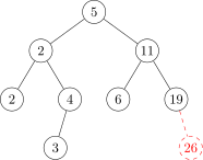
To delete a leaf node, we simply set the link from its parent to null. See the figure above. Here is the code to take care of this case:
if (n.left == null && n.right == null)
{
    if (parent.left == n)
        parent.left = null;
    else
        parent.right = null;
    return;
}
Case 2: Deleting a node with one child
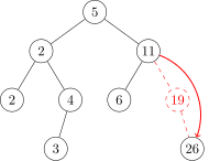
Deleting a node with one child is also pretty straightforward. As shown in the figure above, we simply reroute its parent's link around it to point to its child. The code is a little messy to deal with whether to move left or right links, but it is straightforward. Here it is:
// case 2a: n has a left child and no right child
if (n.right == null)
{
    if (parent.left == n)
        parent.left = n.left;
    else
        parent.right = n.left;
    return;
}

// case 2b: n has a right child and no left child
if (n.left == null)
{
    if (parent.left == n)
        parent.left = n.right;
    else
        parent.right = n.right;
    return;
}
Deleting a node with two children
This is the tricky part because we can't just reroute a link like we did above without potentially messing up the BST property. But there is a clever trick that we can use here that will allow us to preserve the BST property without too much difficulty. What we do is look for the largest value in the node's left subtree and replace the deleted node's value with that value.
For example, suppose we are deleting 9 in the tree below. We would replace 9 with 8, which is the largest value in the left subtree. This will preserve the BST property because (1) we know that 8 is definitely less than anything in 9's right subtree, since 8 came from 9's left subtree, and (2) everything in 9's left subtree will be no larger than 8.
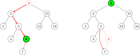
To find the largest value in the left subtree, we step through the left subtree, always following the link to the right until we can't go any farther right. The code to do that is below. Note that we will need to know the parent of the node we find. The code to find the node and its parent is below:
Node m = n.left, parent2 = null;
while (m.right != null)
{
    parent2 = m;
    m = m.right;
}
Once we find the node, we replace n's data value with m's data value. This is simple:
n.data = m.data;
Finally, we have to remove m from the tree. We might have a problem if m itself has two children, but, fortunately, that can't happen. We found m by moving as far right as possible, so we are guaranteed that m has no right child. Therefore, deleting m involves routing its parent's link around it to its child. However, we still have to be careful about how we do this because there is the possibility that m is n's child. In that case, the while loop condition would never have been true and parent2 would be null. We take care of this like below:
if (parent2 == null)
    n.left = m.left;
else
    parent2.right = m.left;
Finally, there is one more thing to worry about, and that is if the value to be removed is stored in the root and the root has 0 or 1 children. These are edge cases that are not handled by our method. So we'll add the following special cases at the beginning of the method:
if (root.data == data && root.left == null)
{
    root = root.right;
    return;
}

if (root.data == data && root.right == null)
{
    root = root.left;
    return;
}
The entire BST class
Here is the entire BST class:
public class BinarySearchTree
{
    private class Node
    {
        int data;
        Node left, right;

        public Node(int data, Node left, Node right)
        {
            this.data = data;
            this.left = left;
            this.right = right;
        }
    }

    private Node root;

    public BinarySearchTree()
    {
        root = null;
    }

    public void add(int data)
    {
        if (root == null)
        {
            root = new Node(data, null, null);
            return;
        }

        Node n = root;
        while (true)
        {
            if (data <= n.data && n.left == null)
            {
                n.left = new Node(data, null, null);
                return;
            }

            else if (data <= n.data)
                n = n.left;

            else if (data > n.data && n.right == null)
            {
                n.right = new Node(data, null, null);
                return;
            }

            else
                n = n.right;
        }
    }

    @Override
    public String toString()
    {
        return toStringHelper(root);
    }

    private String toStringHelper(Node n)
    {
        // in-order traversal
        if (n == null)
            return "";
        return toStringHelper(n.left) + " " + n.data + " " + toStringHelper(n.right);
    }

    public boolean isEmpty()
    {
        return root==null;
    }

    public boolean contains(int data)
    {
        Node n = root;
        while (n != null)
        {
            if (data == n.data)
                return true;
            else if (data <= n.data)
                n = n.left;
            else
                n = n.right;
        }
        return false;
    }

    public void remove(int data)
    {
        // special cases needed if data value to be removed is in root
        // and root has 0 or 1 child
        if (root.data == data && root.left == null)
        {
            root = root.right;
            return;
        }

        if (root.data == data && root.right == null)
        {
            root = root.left;
            return;
        }

        // find the node to be removed
        Node n = root, parent = null;
        while (data != n.data)
        {
            parent = n;
            n = (data > n.data) ? n.right : n.left;
        }

        // case 1: n has no children
        if (n.left == null && n.right == null)
        {
            if (parent.left==n)
                parent.left = null;
            else
                parent.right = null;
            return;
        }

        // case 2a: n has a left child and no right child
        if (n.right == null)
        {
            if (parent.left == n)
                parent.left = n.left;
            else
                parent.right = n.left;
            return;
        }

        // case 2b: n has a right child and no left child
        if (n.left == null)
        {
            if (parent.left == n)
                parent.left = n.right;
            else
                parent.right = n.right;
            return;
        }

        // case 3: n has two children (only remaining case)

        // find the node with the largest value in n's left subtree
        // and find its parent
        Node m = n.left, parent2 = null;
        while (m.right != null)
        {
            parent2 = m;
            m = m.right;
        }

        // set n's data value to m's value
        n.data = m.data;

        // delete m from the tree
        if (parent2 == null)
            n.left = m.left;
        else
            parent2.right = m.left;
    }
}
More about BSTs
An important consideration about BSTs is how well balanced they are. Roughly speaking, a tree is balanced if all of the paths from the root to the leaves (end-nodes) are roughly the same length. If there are some long and some short paths, the tree is unbalanced. In the perfectly balanced case, each of the paths from the root to the leaves has length log n, where n is the number of nodes. In a case like this, the add and contains methods work in O(log n) time as they both walk down the tree one level at a time, until they reach their goal or the bottom of the tree. The remove method will also work in O(log n) time.
Shown below on the left is a perfectly balanced tree. On the right is an unbalanced tree.
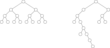
The reason for the appearance of the logarithm in the running times is this: Suppose we have a perfectly balanced BST with n elements in total. At the root level there is one node. At the next level there are two nodes, the root's two children. At the next level, each child has two children for a total of four nodes. In general, as we go from level to the next, the number of nodes doubles, so we have 2k-1 nodes at level k, where level 1 is the root level. If the tree is completely full to level k, then, using the geometric series formula, we find that there are 1+2+4+…+2k-1 = 2k-1 total nodes in the tree. Thus we see that a tree with n nodes and k levels must satisfy the equation 2k-1=n. Solving for k, we get k=log(n+1). So the number of levels is the logarithm of the number of nodes. Another way to look at things is that each time we choose a left or right child and step down the tree, we cutting off half of the tree. This continual dividing in half is just like the binary search algorithm, which has a logarithmic running time.
As long as the tree is relatively balanced, the methods will work in more or less O(log n) time. If there is a lot of data and it's pretty random, the tree will be fairly well balanced. On the other hand, suppose the data we're putting into a BST already happens to be sorted. Then each item as its added to the BST will be added as the right child of its parent. The result is a degenerate tree, a long string of nodes, arranged like in a list. In this case the BST behaves a lot like a linked list and all the operations are reduced to O(n). This is a serious problem because in a lot of real life situations, data is often sorted or nearly sorted.
In a case like this, there are techniques to balance the tree. One of these techniques, AVL trees, involves rebalancing the tree after each addition of a node. This involves moving around a few nodes in the area of the added node. Another technique is red-black trees. These techniques are nice to know, but we will not cover them here. They are covered in other data structures books and on the web.
Java's Comparable interface
We chose to implement the binary search tree only with integer data instead of generics. The reason for this is that we have to compare the data values, and values from any old generic type might not be comparable. But there is a way to use generics here if we use Java's Comparable interface.
First, here is an example of the using the Comparable interface to make the objects of a class comparable. Say we have a class called Record that contains two fields, name and score. Initially, we have no natural way of comparing two of these objects. But, let's say we want to be able to compare them based on the value of score. Here is how to do that:
public class Record implements Comparable<Record>
{
    private String name;
    private int score;

    public Record(String name, int score)
    {
        this.score = score;
        this.name = name;
    }

    @Override
    public String toString()
    {
        return name + ":" + score;
    }

    public int compareTo(Record record)
    {
        return this.score - record.score;
    }
}
We implement the Comparable interface. To do that we have to define a method compareTo that describes how to compare two objects. The method must return either a negative value, 0, or a positive value depending on whether current object is smaller than, equal to, or larger than the object it is being compared to. Here is an example of how to use the Record class:
Record rec1 = new Record("Bob", 88);
Record rec2 = new Record("Sally", 92);

if (rec1.compareTo(rec2) > 0)
    System.out.println("rec1 is larger than rec2.");
To rewrite the binary search tree class using generics, we have only a few changes to make. First, here is the declaration of the class:
public class BinarySearchTreeGeneric<T extends Comparable<T>>
The exact syntax is important here. It basically says that our BST class will be able to work with any class for which a way to compare objects of that class has been defined. Specifically, anything that implements Comparable must have a compareTo method, and that is what our BST class will use. We go through and replace all occurrences of int data with T data and replace comparisons like data < n.data with data.compareTo(n.data) < 0. For example, here is how the contains method changes:
public boolean contains(int data)           public boolean contains(T data)
{                                           {
    Node n = root;                              Node n = root;
    while (n!=null)                             while (n!=null)
    {                                           {
        if (data == n.data)                         if (data.compareTo(n.data) == 0)
            return true;                                return true;
        else if (data < n.data)                      else if (data.compareTo(n.data) < 0)
            n = n.left;                                 n = n.left;
        else                                        else
            n = n.right;                                n = n.right;
    }                                           }
    return false;                               return false;
}                                           }
Here is the entire generic BST.
public class GenericBST<T extends Comparable<T>>
{
    private class Node
    {
        T data;
        Node left, right;

        public Node(T data, Node left, Node right)
        {
            this.data = data;
            this.left = left;
            this.right = right;
        }
    }

    private Node root;

    public GenericBST()
    {
        root = null;
    }

    public void add(T data)
    {
        if (root==null)
        {
            root = new Node(data, null, null);
            return;
        }

        Node n = root;
        while (true)
        {
            if (data.compareTo(n.data) <= 0 && n.left == null)
            {
                n.left = new Node(data, null, null);
                return;
            }

            else if (data.compareTo(n.data) <= 0)
                n = n.left;

            else if (data.compareTo(n.data) >= 1 && n.right == null)
            {
                n.right = new Node(data, null, null);
                return;
            }

            else
                n = n.right;
        }
    }

    @Override
    public String toString()
    {
        return toStringHelper(root);
    }

    private String toStringHelper(Node n)
    {
        // in-order traversal
        if (n == null)
            return "";
        return toStringHelper(n.left) + " " + n.data + " " + toStringHelper(n.right);
    }

    public boolean isEmpty()
    {
        return root==null;
    }

    public boolean contains(T data)
    {
        Node n = root;
        while (n != null)
        {
            if (data.compareTo(n.data) == 0)
                return true;
            if (data.compareTo(n.data) >= 1)
                n = n.right;
            else
                n = n.left;
        }
        return false;
    }

    public void remove(T data)
    {
        // special cases needed if data value to be removed is in root
        // and root has 0 or 1 child

        if (root.data.compareTo(data) == 0 && root.left == null)
        {
            root = root.right;
            return;
        }

        if (root.data.compareTo(data) == 0 && root.right == null)
        {
            root = root.left;
            return;
        }

        // find the node to be removed
        Node n = root;
        Node parent = null;
        while (data != n.data)
        {
            parent = n;
            if (data.compareTo(n.data) >= 1)
                n = n.right;
            else
                n = n.left;
        }

        // case 1: n has no children
        if (n.left == null && n.right == null)
        {
            if (parent.left == n)
                parent.left = null;
            else
                parent.right = null;
            return;
        }

        // case 2a: n has a left child and no right child
        if (n.right == null)
        {
            if (parent.left == n)
                parent.left = n.left;
            else
                parent.right = n.left;
            return;
        }

        // case 2b: n has a right child and no left child
        if (n.left == null)
        {
            if (parent.left == n)
                parent.left = n.right;
            else
                parent.right = n.right;
            return;
        }

        // case 3: n has two children (only remaining case)

        // find the node with the largest value in n's left subtree
        // and find its parent
        Node m = n.left;
        Node parent2 = null;
        while (m.right != null)
        {
            parent2 = m;
            m = m.right;
        }

        // set n's data value to m's value
        n.data = m.data;

        // delete m from the tree
        if (parent2 == null)
            n.left = m.left;
        else
            parent2.right = m.left;
    }
}
Here is an example test of the class using strings:
GenericBST<String> bst = new GenericBST<String>();

bst.add("e");
bst.add("a");
bst.add("o");
bst.add("u");
bst.add("i");

System.out.println(bst);
a e i o u
Here is an example test of the class using the Record class from earlier in the section.
GenericBST<Record> bst = new GenericBST<Record>();

List<String> names  = new ArrayList<String>();
List<Integer> scores = new ArrayList<Integer>();

Collections.addAll(names, "Al", "Bob", "Carol", "Deb", "Elly");
Collections.addAll(scores, 88, 77, 68, 95, 56);

for (int i=0; i<names.size(); i++)
    bst.add(new Record(names.get(i), scores.get(i)));
System.out.println(bst);
Elly:56 Carol:68 Bob:77 Al:88 Deb:95
Java's Collections Framework does not have a dedicated BST class, though it does use BSTs to implement some other data structures (like sets and maps, which we'll see in a future chapter).
Heaps
A heap is a relative of a BST. Like BSTs, heaps maintain their elements in a kind of sorted order. The main property of heaps is that they are a way to store data in which continually finding and possibly removing the smallest element is designed to be very fast. In particular, finding the minimum element in a heap is a O(1) operation, compared with O(log n) for a BST. However, unlike BSTs, heaps do not store all the data in sorted order. It's just the minimum value that is guaranteed to be easy to find.
The definition of a heap is that it is a binary tree with two special properties:
- The value of a parent node is less than or equal to the values of both its children.
- The nodes are entered in the tree in the order shown in the figure below. Start at the root and work down the tree from left to right, typewriter style, completely filling a level before moving on to the next.
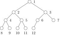
Notice the difference in property 1 between BSTs and heaps. In a BST, values to the left of the parent are always less than or equal to the parent's value and values to the right are larger, whereas in a heap, left and right are not important. All that matters is that the values of the parent be less than or equal to the values of its children. Property 2 guarantees that the heap is a balanced binary tree.
The heap described above is a min-heap. We can also have a max-heap, where the “less than” in property 1 is changed to “greater than.”
Implementing a heap
Looking at the heap shown above, we notice an interesting relationship between the parent and its left child. The “index” of the left child is exactly twice the “index” of the parent. Because of this and the fact the tree has no gaps, we can implement a heap with a dynamic array instead of as a linked structure with nodes. In particular, the root will be at list index 0, its two children will be at indices 1 and 2, its left child's children will be at indices 3 and 4, etc. The figure below shows the indices of the nodes in the heap.
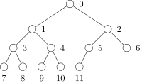
This is the same as the first figure in this section, but with all the indices shifted by 1. The relationship we noted between parents and children still holds, more or less. In particular, if p is the index of the parent, then its children are at indices 2p+1 and 2p+2. Shown below is an example heap and its dynamic array representation:
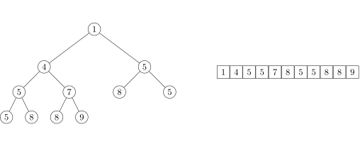
Here is the start of the class. For simplicity, we will assume the heap's data are integers. Later, we will rewrite it using generics.
public class Heap
{
    private List<Integer> data;

    public Heap()
    {
        data = new ArrayList<Integer>();
    }
}
Adding to a heap
When we add an item to a heap, we have to make sure it is inserted in a spot that maintains the heap's two properties. To do this, we first insert it at the end of the heap. This takes care of the second property (completely filling the heap left to right, typewriter style), but not necessarily the first property (parent's data less than or equal to its children's data). To take care of that, we compare the inserted value with its parent. If it is less than its parent, then we swap child and parent. We then compare the inserted value to the parent's parent and swap if necessary. We keep moving upward going until the first property is satisfied or until we get to the root. The new item sort of bubbles up until it gets into a suitable place in the heap.
Here is an example where we add the value 3 (shown in green) to the heap. We start by placing it at the end of the heap. Its value is out of place, however. We compare its value to its parent, which has value 8. Since 3<8, a swap is necessary. We then compare 3 with its new parent, which has value 5. Since 3<5, another swap is needed. We again compare 3 with its new parent and this time 3>1, so we can stop.
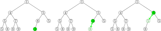
Here is the code for the method:
public void add(int value)
{
    data.add(value);
    int c = data.size()-1, p = (c-1)/2;
    while (data.get(c) < data.get(p))
    {
        int hold = data.get(p);
        data.set(p, data.get(c));
        data.set(c, hold);
        c = p;
        p = (c-1)/2;
    }
}
The code is a direct implementation of the preceding discussion. The only thing worth mentioning is how to use the child's index in the list to find its parent's index. If the parent's index is p, then we know its children are located at c1=2p+1 and c2=2p+2. Solving each of these for p, we get p=(c1-1)/2 and (c2-2)/2. But the code has just the formula (c-1)/2 that works for both children. The reason for this is that the division is integer division. For example, if p=4, its children are at c1=9 and c2=10, and using the formula from the code, we get (9-1)/2 =4 and (10-1)/2=4, so one formula actually covers both cases because of the floor operation implicit in the division.
Removing the top of the heap
The other important heap operations are peek and pop. The peek method returns the value of the minimum element in the heap. Since that value is always stored at the top of the heap, this is an easy thing to do:
public int peek()
{
    return data.get(0);
}
The pop method not only returns the minimum value in the heap, but it also removes it from the heap. This is a little tricky because we have to move things around in the heap to fill in the gap left by removing the top. The idea here is similar to what we did with adding an element, just done in reverse. What we do is take the last element, x, in the heap and move it to the top. This ensures that property 2 is satisfied. But doing so will probably break property 1, so we compare x with its children and swap if necessary. We then compare x with its new children and swap again if necessary. We continue this until property 1 is satisfied. Essentially, the item sinks until it is at a suitable place in the heap. Note that when doing the comparisons, we always swap with the smaller of the two children to ensure that property 1 holds. Here is an example:
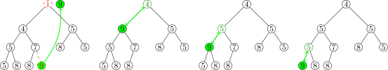
Here is the code for the method:
public int pop()
{
    // remove the top entry and replace it with the last entry

    int saveFirst = data.get(0);
    data.set(0, data.get(data.size()-1));
    data.remove(data.size()-1);

    // bubble the new top down to its proper place in the tree

    int p = 0, c1=2*p+1, c2=2*p+2;
    while (c2<data.size() &&  (data.get(p)>data.get(c1) || data.get(p)>data.get(c2)))
    {
        if (data.get(c1) > data.get(c2))
        {
            int hold = data.get(p);
            data.set(p, data.get(c2));
            data.set(c2,  hold);
            p = c2;
        }
        else
        {
            int hold = data.get(p);
            data.set(p, data.get(c1));
            data.set(c1,  hold);
            p = c1;
        }
        c1 = 2*p+1;
        c2 = 2*p+2;
    }

    // special case if a swap needs to be made at end of tree where parent has
    // a left child but no right child

    if (c2==data.size() && data.get(p)>data.get(c1))
    {
        int hold = data.get(p);
        data.set(p, data.get(c1));
        data.set(c1,  hold);
    }

    return saveFirst;
}
The method starts by saving the value of the top of the tree for the return statement at the end of the function. Then we remove the last element from the heap and use it to replace the top element.
We then step through the tree looking for where to place the new value. The loop is set to run until we either reach the end of the tree or find a suitable position. At each step of the loop, we check to see if the value is greater than either of its children's values and swap if so. The condition on the first if statement, p>c1 && c1<=c2, guarantees that we will swap with the smaller child. If the value is not greater than either child, then property 1 is satisfied and we stop looping.
Other than that, there is one special case to consider, which is if the parent has a left child at the end of the tree and no right child. Since there is no right child, the loop will have ended, so we need this special case after the loop to see if the parent and left child should be swapped.
Making the class generic
Just like with BSTs, since we are comparing values, to use generics we use the Comparable interface. Mostly this just involves replacing things like p>c2 with p.compareTo(c2)>0, similarly to how we made the BST class generic. However, we can take things a little further. If we want to make our heap a max-heap, where the parent is always greater than or equal to its children (and the root stores the maximum value instead of the minimum), the only changes we need to make are to reverse all the greater than and less than symbols. For instance, p>c2 becomes p≤c2, or with generic code it becomes p.compareTo(c2)>0 becomes p.compareTo(c2)<0.
It seems like a waste to copy and paste all the code to create a max-heap class when all we have to change is a few symbols, and, fortunately, there is a better way. Here is the trick: the expression a<0 is equivalent to -a>0. This seemingly trivial algebraic fact will make it so that we don't have to change any of the < and > symbols in our code. Instead, we will create a class variable, called heapType that is set to 1 or -1 depending on whether we have a min-heap or max-heap and use this trick, like in the examples below. On the left below are two conditions and on the right is what they will change to.
p > c2               p.compareTo(c2)*heapType > 0
c1 <= c2             c1.compareTo(c2)*heapType <= 0
Below is the code for the generic heap class. For convenience, we have also added a toString method and an isEmpty method.
import java.util.List;
import java.util.ArrayList;

public class Heap<T extends Comparable<T>>
{
    public static final int MAXHEAP=-1, MINHEAP=1;
    private int heapType;

    private List<T> data;

    public Heap(int heapType)
    {
        data = new ArrayList<T>();
        this.heapType = heapType;
    }

    public void add(T value)
    {
        data.add(value);
        int c = data.size()-1, p = (c-1)/2;
        while (data.get(c).compareTo(data.get(p))*heapType < 0)
        {
            T hold = data.get(p);
            data.set(p, data.get(c));
            data.set(c, hold);
            c = p;
            p = (c-1)/2;
        }
    }

    public T peek()
    {
        return data.get(0);
    }

    public T pop()
    {
        // remove the top entry and replace it with the last entry

        T saveFirst = data.get(0);
        data.set(0, data.get(data.size()-1));
        data.remove(data.size()-1);

        // bubble the new top down to its proper place in the tree

        int p = 0, c1=2*p+1, c2=2*p+2;
        while (c2<data.size() &&
              (data.get(p).compareTo(data.get(c1))*heapType > 0
               || data.get(p).compareTo(data.get(c2))*heapType > 0))
        {
            if (data.get(c1).compareTo(data.get(c2))*heapType > 0)
            {
                T hold = data.get(p);
                data.set(p, data.get(c2));
                data.set(c2,  hold);
                p = c2;
            }
            else
            {
                T hold = data.get(p);
                data.set(p, data.get(c1));
                data.set(c1,  hold);
                p = c1;
            }
            c1 = 2*p+1;
            c2 = 2*p+2;
        }

        // special case if a swap needs to be made at end of tree where parent has
        // a left child but no right child

        if (c2==data.size() && data.get(p).compareTo(data.get(c1))*heapType > 0)
        {
            T hold = data.get(p);
            data.set(p, data.get(c1));
            data.set(c1,  hold);
        }

        return saveFirst;
    }

    public boolean isEmpty()
    {
        return data.isEmpty();
    }

    @Override
    public String toString()
    {
        return data.toString();
    }
Here is a simple test of the class. It will print out the strings in alphabetical order.
Heap<String> heap = new Heap<String>(Heap.MINHEAP);
heap2.add("abc");
heap2.add("wxy");
heap2.add("def");
System.out.println(heap.pop());
System.out.println(heap.pop());
System.out.println(heap.pop());
Here is another test of the class. This one puts 50 random integers into the heap and then pops them all off. The integers will be popped off in increasing order.
Heap<Integer> heap = new Heap<Integer>(Heap.MINHEAP);
Random random = new Random();

for (int i=0; i<50; i++)
    heap.add(random.nextInt(100));

for (int i=0; i<50; i++)
    System.out.print(heap.pop() + " ");
Running time and applications of heaps
Running time of the methods
The peek method, which returns (but does not remove) the minimum value of a min-heap, is O(1). This is because the minimum value is always stored at the top of the heap and it is a quick data.get(0) to return that value.
The add and pop methods of heaps each run in O(log n) time. In the worst case scenario, each method will require a number of swaps equal to the number of levels in the tree. The heap is a complete binary tree, so the number of levels is the logarithm of the number of nodes in the tree.
Since the add method runs in O(log n) time, building a heap from a list n elements will run in O(nlog n) time. (There does exist an O(n) algorithm for doing that, but it is beyond the scope of this book.)
Applications of heaps
As we saw in the examples at the end of the last section, repeatedly popping elements off of the heap returns the values in order. So heaps can be used to sort data. This sort is called Heapsort and it is one of the faster sorts out there. We will have more to say about it in the sorting chapter. Heaps are also used to implement certain graph algorithms in this chapter. In general, heaps are useful when you are continually adding things to a data structure and need quick access to the smallest or largest value added.
Just like with BSTs, Java's Collections Framework does not have a dedicated heap class, but it does use heaps to implement other data structures. In fact, this section shows how to use one of those data structures, called a priority queue, as a heap.
Priority Queues
A priority queue is a data structure related to a queue. The difference is that each element is given a priority and when elements are removed from the queue, they are removed in order of priority. Lots of real-life situations can be described by priority queues. For instance, in our everyday lives we have a bunch of things to do, some of which have higher priorities than others. In computers, operating systems use priority queues to determine which tasks to run when, as certain tasks are more important than others.
Implementing a priority queue
Heaps provide a straightforward and efficient way to implement a priority queue. Our priority queue class will have four methods:
-
enqueue— takes an item and its priority and puts the item onto the queue based off its priority -
dequeue— removes and returns the highest priority item -
peek— returns the value of the highest priority item without removing it -
isEmpty— returnstrueorfalsedepending on whether the queue is empty or not
There is one trick here. We want the heap to sort things based on their priority. To do this, we will create a subclass called PQItem that has two fields: the data and its priority. The class will implement Comparable and compare PQItem objects based off their priority field.
Implementing the priority queue methods is very quick since we will use a heap to do all the work. We will have one class variable, heap, which is of type Heap<PQItem>. Each of our four methods will simply call the appropriate heap method. Here is the entire class.
public class PQueue<T>
{
    private class PQItem implements Comparable<PQItem>
    {
        public T data;
        public int priority;

        public PQItem(T data, int priority)
        {
            this.data = data;
            this.priority = priority;
        }

        public int compareTo(PQItem other)
        {
            return this.priority - other.priority;
        }
    }

    private Heap<PQItem> heap;

    public PQueue()
    {
        heap = new Heap<PQItem>(Heap.MAXHEAP);
    }

    public void enqueue(T data, int priority)
    {
        heap.add(new PQItem(data, priority));
    }

    public T dequeue()
    {
        return heap.pop().data;
    }

    public T peek()
    {
        return heap.peek().data;
    }

    public boolean isEmpty()
    {
        return heap.isEmpty();
    }
}
Here is a small example of how to use it:
Q.enqueue("Low priority event", 1);
Q.enqueue("High priority event", 8);
Q.enqueue("Medium priority event", 5);
Q.enqueue("Super high priority event", 10);

System.out.println(Q.dequeue());
System.out.println(Q.dequeue());
System.out.println(Q.dequeue());
System.out.println(Q.dequeue());
Super high priority event
High priority event
Medium priority event
Low priority event
Applications of priority queues
The take-home message is that heaps and priority queues are useful whenever we are continually storing data and need quickly retrieve the smallest or largest values stored so far. One place this is important is in implementing some useful algorithms like Dijkstra's shortest path algorithm, Prim's algorithm, and the A* search algorithm.
Priority queues are useful in a number of other algorithms. Here's one example: Suppose we have a list of integers and we want a function that returns a list of the n largest integers. One way to get them is to sort the list and then return the last n elements of the sorted list. But what if we are reading a lot of data, say from a file, and there is too much data to put into a list without running out of memory? We need a different approach. One such approach is to use a priority queue. As we read the data from the file, we add it to the priority queue, and once the queue has n elements in it, we start popping things off the queue. At each step, the minimum value is popped off, leaving us with only the n largest. One of the exercises in this chapter is about this.
Here's one more example of priority queues. An important type of simulation is simulating a large number of particles that can collide with one another. This shows up in computer games and in simulations of molecules, among other places. Let's say we have n particles. Usually simulations work by setting a small time step, say .001 seconds, and at every time step we advance all the particles forward by the appropriate amount. At each time step we then have to check for collisions. One way to go about checking for collisions is to loop through the particles and for each particle, loop through the other particles, checking to see which are about to collide with the current particle. This requires a total of n(n-1)/2 checks. This is a lot of checks to be making every .001 seconds.
We can greatly reduce the number of checks using a priority queue. The way this approach works is as follows: First assume that the particles are moving in straight line trajectories. We can calculate ahead of time when two particles will collide. We then use a priority queue of collisions, with priority given by the collision time. After each time step we pop off any imminent collisions from the queue and address them. It may happen that a collision we calculated ahead of time may not happen because one of the particles got deflected in the meantime, so we also keep track of which collisions won't happen. After addressing collisions, we have to recalculate new collisions since the colliding particles are now moving in different directions, but the total number of these calculations is usually a lot less than n(n-1)/2.
Priority queues and heaps in the Collections Framework
The Collections Framework has an interface called PriorityQueue and a class called PriorityQueue implementing it. It has the following methods, which are the same as for ordinary queues:
| Method | Description |
|---|---|
add | add something to the queue |
remove | remove something from the queue |
element | returns the next thing to come off the queue without removing it |
Here is an example of using PriorityQueue to schedule events, like in the previous section. To do so, we will create a new class PQItem. It is essentially the same as the one from the previous section.
public class PQItem<T> implements Comparable<PQItem<T>>
{
    private T data;
    private int priority;

    public PQItem(T data, int priority)
    {
        this.data = data;
        this.priority = priority;
    }

    public T getData()
    {
        return data;
    }

    public int compareTo(PQItem<T> other)
    {
        return this.priority - other.priority;
    }
}
Here is the PriorityQueue tester:
PriorityQueue<PQItem<String>> pq = new PriorityQueue<PQItem<String>>();

pq.add(new PQItem<String>("Low priority event", 1));
pq.add(new PQItem<String>("High priority event", 8));
pq.add(new PQItem<String>("Medium priority event", 5));
pq.add(new PQItem<String>("Super high priority event", 10));

System.out.println(pq.remove().getData());
System.out.println(pq.remove().getData());
System.out.println(pq.remove().getData());
System.out.println(pq.remove().getData());
PriorityQueue can be used with any class that implements Comparable. The remove method will remove things in the order based on the class's compareTo method. As a simple example, Java's String class implements Comparable, comparing strings alphabetically. The following code puts a few strings onto the queue and they are removed in alphabetical order. It prints out ACX.
PriorityQueue<String> Q = new PriorityQueue<String>();
Q.add("C");
Q.add("X");
Q.add("A");
System.out.println(Q.remove() + Q.remove() + Q.remove());
To get the queue to work in reverse, we can define our own comparator and pass it as an argument to the priority queue constructor. This constructor also requires us to specify the initial capacity of the queue. Here is the code. It prints out XCA.
PriorityQueue<String> P = new PriorityQueue<String>(
                           new Comparator<String>() {
                            public int compare(String x, String y) {
                             return y.compareTo(x);}});
P.add("C");
P.add("X");
P.add("A");
System.out.println(P.remove() + P.remove() + P.remove());
The comparator we define is an example of an anonymous class in Java. Further, to keep the comparison code short, we piggyback off of the String class's comparator, but it reverse the order (y.compareTo(x)) to cause things to work in reverse. In Java 8 and later, there is a shortcut to creating the anonymous class. Here it is:
PriorityQueue<String> P = new PriorityQueue<String>((x,y) -> y.compareTo(x));
Note: According to Java's documentation, the remove method of PriorityQueue runs in O(n) time, not O(log n) time.
Heaps
Heaps and priority queues are very similar, and we can use Java's PriorityQueue class as a heap. Here is how to use it with the same test program as the one we wrote to test our own heap class.
PriorityQueue<Integer> heap = new PriorityQueue<Integer>();
Random random = new Random();

for (int i=0; i<10; i++)
    heap.add(random.nextInt(30));
System.out.println(heap);

for (int i=0; i<10; i++)
    System.out.print(heap.remove() + " ");
Exercises
- The following elements are added to a binary search tree in the order given.
[16, 10, 24, 4, 9, 13, 22, 30, 23, 11, 14, 4]
- Draw what the tree will look like after everything has been added.
- The element 22 is removed. Draw what the tree looks like now.
- The element 10 is removed. Draw what the tree looks like now.
- The following elements are added to a heap in the order given.
[16, 10, 24, 4, 9, 13, 22, 30, 23, 11, 14, 4]
- Draw what the heap will look like after everything has been added.
- The top is removed. Draw what the heap looks like now.
- The new top is removed. Draw what the heap looks like now.
- In your own words, carefully explain why, when deleting a node with two children, we replace it with the largest element in its left subtree. In particular, why does that element preserve the binary search tree property?
- This exercise involves adding some methods to the BST class. Your methods must make use of the order property of binary search trees. In other words, they should work with binary search trees, but not on an arbitrary binary tree. A method that has to look at every node in the tree, regardless of the input data, is not good enough here. Binary search trees are ordered to make searching faster than with arbitrary trees and this problem is about taking advantage of that ordering.
-
min()— returns the minimum item in the BST -
max()— returns the maximum item in the BST -
get(k)— returns the kth smallest item in the BST -
numberLess(n)— returns the number of elements in the tree whose values are less thann. Do not use thetoArrayListmethod from the next exercise. -
successor(x)— returns the next largest item in the tree greater than or equal tox. Throw an exception if there is no such item. -
toArrayList()— returns an ArrayList containing the elements of the tree in increasing order
-
- Add the following methods to the
Heapclass:-
size()— returns the number of elements in the heap -
delete(x)— Deletes an arbitrary elementxfrom the heap. One way to do this is to do a linear search through the list representing the heap until you find the element and then delete it in more or less the same way to how thepopmethod removes the min. If there are multiple copies ofx, your method doesn't have to delete all of them. -
isHeap(list)— a static method that takes a list as a parameter and returnstrueorfalsedepending on if the list could represent a heap. Recall from class how we converted between the binary tree representation of a heap and a list representation. To write this method, you just have to verify that in the list, each parent's value is always less than or equal to its childrens' values. Recall that the children of the node at list index p are located at indices 2p+1 and 2p+2. -
numberOfPCCMatches()— returns how many nodes in the heap have the same values as both of their children.
-
- Suppose we have a list of integers and we want a function that returns a list of the n largest integers. One way to get them is to sort the list and then return the last n elements of the sorted list. But what if we are reading a lot of data, say from a file, and there is too much data to put into a list without running out of memory? We need a different approach. One such approach is to use a priority queue. As we read the data from the file, we add it to the priority queue and once the queue has n elements in it, we start popping things off the queue. At each step, the minimum value is popped off, leaving us with only the n largest. Write a method whose parameters are a data file (or file name) and an integer
n. Assume the data file contains integer data. The method should use the approach described here to find thenlargest values in the file. - Do the same as the previous exercise, but find the
nsmallest values.
Sets, Maps and Hashing
This chapter is about two useful data structures—sets and maps—and a useful technique called hashing that we will use to implement those data structures.
Sets
A set is a collection of objects with no repeats. Common operations with sets A and B include the union, A ∪ B, which consists of all the elements in A or B (or both); the intersection, A ∩ B, which consists of all the elements in both A and B; and the difference A - B, which consists of all the elements of A that are not in B.
We will first implement a set in a simple and natural way, using a list to hold its data. It will be quick to code and understand, but it will not be very efficient. However, it's good practice to try implementing a set like this before we get to a more sophisticated method later in the chapter. Here is the beginning of the class.
public class SimpleSet<T>
{
    private List<T> data;

    public SimpleSet()
    {
        data = new ArrayList<T>();
    }
}
Here is the add method for adding things to the set. The important thing here is that a set can't have repeats, so before adding an element, we to make sure it is not already in the set.
public void add(T x)
{
    if (!data.contains(x))
        data.add(x);
}
Here is another constructor that creates a set from a list by calling our class's add method for each element of the list:
public SimpleSet(List<T> list)
{
    data = new ArrayList<T>();
    for (T x : list)
        this.add(x);
}
The running time of this algorithm can be O(n2), which is not ideal. We get a factor of n because we loop through the entire list and another factor of n (on average) from the contains method.
Next, we can implement remove, toString, size, isEmpty, and contains methods very quickly just by piggybacking off of the ArrayList methods of the same name. For example, here is the toString method (the others are implemented similarly).
@Override
public String toString()
{
    return data.toString();
}
We also have a method that returns the data of the set as a list. Here it is:
public List<T> getData()
{
    return new ArrayList<T>(data);
}
Note that we don't just return data as then any changes the caller makes to returned list will affect data itself. Instead we make a copy of the list and return that. There is still one problem that we won't address here. This returns a shallow copy of the list. If the elements in data are mutable objects, the caller can still change them.
Union, intersection, and difference
With this approach to sets it is straightforward to implement union, intersection, and difference. For union, we create an empty set, add the values from data, then add the values from the second set. The add method will make sure there are no repeats.
public SimpleSet<T> union(SimpleSet<T> set2)
{
    SimpleSet<T> returnSet = new SimpleSet<T>();

    for (T x : data)
        returnSet.add(x);

    for (T x : set2.data)
        returnSet.add(x);

    return returnSet;
}
The intersection method works somewhat similarly to union. What we do here is create an empty set, loop through the data of the second set and only add those values that are also in data. The difference method is very similar, the main difference being we loop through data and only add things that are not in the second set.
The entire class
Here is the entire class:
import java.util.ArrayList;
import java.util.List;

public class SimpleSet<T>
{
    private List<T> data;

    public SimpleSet()
    {
        data = new ArrayList<T>();
    }

    public SimpleSet(List<T> list)
    {
        data = new ArrayList<T>();
        for (T x : list)
            if (!data.contains(x))
                data.add(x);
    }

    @Override
    public String toString()
    {
        return data.toString();
    }

    public int size()
    {
        return data.size();
    }

    public boolean isEmpty()
    {
        return data.isEmpty();
    }

    public boolean contains(T x)
    {
        return data.contains(x);
    }

    public List<T> getData()
    {
        List<T> returnList = new ArrayList<T>();
        for (T x : data)
            returnList.add(x);
        return returnList;
    }

    public void add(T x)
    {
        if (!data.contains(x))
            data.add(x);
    }

    public void remove(T x)
    {
        data.remove(x);
    }

    public SimpleSet<T> union(SimpleSet<T> set2)
    {
        SimpleSet<T> returnSet = new SimpleSet<T>();

        for (T x : data)
            returnSet.add(x);

        for (T x : set2.data)
            returnSet.add(x);

        return returnSet;
    }

    public SimpleSet<T> intersection(SimpleSet<T> set2)
    {
        SimpleSet<T> returnSet = new SimpleSet<T>();

        for (T x : data)
            if (set2.contains(x))
                returnSet.add(x);

        return returnSet;
    }

    public SimpleSet<T> difference(SimpleSet<T> set2)
    {
        SimpleSet<T> returnSet = new SimpleSet<T>();

        for (T x : data)
            if (!set2.contains(x))
                returnSet.add(x);

        return returnSet;
    }
}
Analysis of running time
The methods here are pretty slow. They are fine for small data sets, but they don't scale well. The add method is O(n) because it uses the ArrayList contains method, which is O(n). That method essentially has to loop through the list to see if a value is in the list. The constructor that builds a set from a list runs in more or less O(n2) time, as it loops through the list and calls the O(n) add method at each step. The union method is O(n2+m2), where n and m are the sizes of the two sets, as the method consists of a loop with a call to the add method inside. The intersection is even worse, being cubic in the worst case (specifically O(n2m)). It consists essentially of three nested loops, namely a loop over all n elements of the set, with a call to contains nested inside (which loops over the m-elements of set2) and a call to add inside the if statement (which has to loop again over the n elements of the set to check for repeats).
The next section is about hashing, a technique that will give us O(1) add and remove methods and bring the other operations down to O(n).
Hashing
Consider first the following approach to implementing a set: Suppose we know our set will only consist of integers from 0 to 999. We could create a list, called data, consisting of 1000 booleans. If the ith entry of data is true, then i is in the set and otherwise it's not. Inserting and deleting elements comes down to setting a single element of data to true or false, an O(1) operation. Checking if the set contains a certain element comes down to checking if the corresponding entry in data is true, also an O(1) operation. This will also bring down the union, intersection, and difference operations down to linear time.
This type of set is called a bit set and it is the subject of an exercise in this chapter. This approach has a problem, though. If our set could consist of any 32-bit integer, then we would need an ArrayList of about four billion booleans, which is not practical.
Suppose, however, that we do the following: when adding an integer to the set, mod it by 1000, use that result as the integer's index into a list and store that integer at the index. For instance, to add 123456 to the set, we compute 123456 mod 1000 to get 456, and store 123456 at index 456 of the list. This is an example of hashing.
In general, a hash function is a function that takes data and returns a value in a restricted range. For instance, the hash function h(x) = x mod 1000 takes any integer and returns a value in the range from 0 to 999. One immediate problem with this approach is that collisions are possible. This is where different integers end up with the same hash. For example, 123456, 1456, and 10456 all yield the same value when modded by 1000. Collisions with hash functions are pretty much unavoidable, so we need to find a way to deal with them.
There are several approaches. We will focus here on the approach called chaining. Here is how it works: Since several items could hash to the same index, instead of storing a single item at that index, we will store a list of items there. These lists are called buckets. For example, let's say we are using the simple hash function h(x)=x mod 5 and we add 2, 9, 14, 12, 6, and 29 to the set. The hash table will look like this:
0: []
1: [6]
2: [2, 12]
3: []
4: [9, 14, 29]
To add a new element to the set, we run it through the hash function and add it to the list at the resulting index. To determine if the set contains an element, we compute its hash and search the corresponding list for the element.
Hash functions
The hash functions we have considered thus far consist of just modding by a number. This isn't ideal as it tends to lead to a lot of collisions with real-life data. We want to minimize collisions. A good hash function to use with integers is one of the form h(x)=ax mod b, where a and b are relatively large primes.
We can also have hash functions that operate on other data types, like strings. For instance, a simple, but not particularly good, hash function operating on strings of letters might convert the individual letters into numerical values, add the numerical values of the letters, and then mod by 100. For example, the hash of "message" would be 13+5+19+19+1+7+5 mod 100 = 69. Notice how it takes any string and converts it into a value in a fixed range, in this case the range from 0 to 99.
There is a lot that goes into constructing good hash functions. There are many places to learn more about this if you are interested.
Implementing a set with hashing
In this section we will implement a very basic integer set using hashing. First, we need a hash function. Here is a simple one:
public int hashfunc(int key)
{
    return 7927*key % 17393;
}
As mentioned earlier, a good hash function to use with integers is one of the form h(x)=ax mod b, where a and b are relatively large primes. In this case, we picked a=7927 (the 1000th prime) and b=17393 (the 2000th prime). Since we are modding by 17393, we will have that many buckets in our hash table.
The class has two fields, an integer numElements that keeps track of the size of the set, and the list of buckets, called data. It is a list of lists, declared like this:
private List<List<Integer>> data;
Below is the constructor that creates an empty set. It creates the list of buckets. Each element of that list is a list itself and needs to be created before we can add stuff to it.
public HSet()
{
    data = new ArrayList<List<Integer>>(17393);
    for (int i=0; i<17393; i++)
        data.add(new ArrayList<Integer>());
}
The number of buckets will be fixed and cannot be changed. A better approach, such as the one used by the HashSet class in the Java Collections Framework, would be to resize the hash table if things get too full.
We will implement most of the set methods in a very similar way to our simple set implementation from earlier, just with an added hashing step. To add an item to the set, we compute its hash and insert it into the bucket at the hash's index in data. Sets cannot have repeats, so before adding an item to the bucket, we make sure it is not already there.
public void add(int x)
{
    int hash = hashfunc(x);

    if (!data.get(hash).contains(x))
    {
        data.get(hash).add(x);
        numElements++;
    }
}
Removing items from the set is quick:
public void remove(int x)
{
    data.get(hashfunc(x)).remove(x);
    numElements--;
}
The contains method is also quick:
public boolean contains(int x)
{
    return data.get(hashfunc(x)).contains(x);
}
Because we have a class variable keeping track of the number of elements, the isEmpty and size methods are simple:
public boolean isEmpty()
{
    return numElements==0;
}

public int size()
{
    return numElements;
}
Most of the rest of the methods we implement require a way to get a list of the set's elements. Here is a method to do that. It loops through each of the lists that comprise data, adding each of their elements to a master list that is returned.
public List<Integer> getData()
{
    List<Integer> returnList = new ArrayList<Integer>();
    for (List<Integer> list : data)
        for (int x : list)
            returnList.add(x);
    return returnList;
}
Armed with this method, the toString method is simple:
@Override
public String toString()
{
    return this.getData().toString();
}
The union, intersection, and difference methods work much like the method from our earlier implementation of sets. Here is the union method. It makes use of the getData method.
public HSet union(HSet set2)
{
    HSet returnSet = new HSet();

    for (int x : this.getData())
        returnSet.add(x);

    for (int x : set2.getData())
        returnSet.add(x);

    return returnSet;
}
Here is the entire class:
import java.util.ArrayList;
import java.util.List;

public class HSet
{
    private List<List<Integer>> data;
    private int numElements;

    public int hashfunc(int key)
    {
        return 7927*key % 17393;  // 1000th and 2000th primes
    }

    public HSet()
    {
        data = new ArrayList<List<Integer>>(17393);
        for (int i=0; i<17393; i++)
            data.add(new ArrayList<Integer>());
        numElements = 0;
    }

    public HSet(List<Integer> list)
    {
        data = new ArrayList<List<Integer>>(17393);
        for (int i=0; i<17393; i++)
            data.add(new ArrayList<Integer>());
        numElements = 0;

        for (int x : list)
        {
            this.add(x);
            numElements++;
        }
    }

    public void add(int x)
    {
        int hash = hashfunc(x);

        if (!data.get(hash).contains(x))
        {
            data.get(hash).add(x);
            numElements++;
        }
    }

    public void remove(int x)
    {
        data.get(hashfunc(x)).remove(x);
        numElements--;
    }

    public boolean contains(int x)
    {
        return data.get(hashfunc(x)).contains(x);
    }

    public boolean isEmpty()
    {
        return numElements==0;
    }

    public int size()
    {
        return numElements;
    }

    public List<Integer> getData()
    {
        List<Integer> returnList = new ArrayList<Integer>();
        for (List<Integer> list : data)
            for (int x : list)
                returnList.add(x);
        return returnList;
    }

    @Override
    public String toString()
    {
        return this.getData().toString();
    }

    public HSet union(HSet set2)
    {
        HSet returnSet = new HSet();

        for (int x : this.getData())
            returnSet.add(x);

        for (int x : set2.getData())
            returnSet.add(x);

        return returnSet;
    }

    public HSet intersection(HSet set2)
    {
        HSet returnSet = new HSet();

        for (int x : set2.getData())
            if (this.contains(x))
                returnSet.add(x);

        return returnSet;
    }

    public HSet difference(HSet set2)
    {
        HSet returnSet = new HSet();

        for (int x : this.getData())
            if (!set2.contains(x))
                returnSet.add(x);

        return returnSet;
    }
}
More about hashing
The approach we have taken here to deal with collisions is called chaining. If the hash function is a good one, then things will be well spread out through the list and none of the buckets will be very full. In this case, the add and remove methods will run in O(1) time. With a poorly chosen hash function, or if we have a lot of data values and too few buckets, things could degenerate to O(n) time, as we would waste a lot of time when inserting and deleting things from the buckets.
An important consideration in using a hash table is the load factor, which is computed by N/M, where M is the number of buckets and N is the number of elements in the set. As mentioned, if N is large and M is small (a high load factor), then things could degenerate to O(n). If things are reversed—if there are a lot of buckets but the set is small—then there will be few collisions, but lots of wasted space, and iterating through the set will be slowed. Generally, a load factor between about .6 and .8 is considered good.
There is a common alternative to chaining called probing or open addressing. Instead of using lists of elements with the same hash, (linear) probing does the following: Calculate the item's hash. If there is already an element at that hash index, then check the next index in the list. If it is empty, then store the item there, and otherwise keep going until a suitable index is found. There are pros and cons to probing that we won't get into here. More information can be found in other books on data structures or on the web.
Maps
A map is a data structure that is a generalization of a list, where indices may be objects other than integers, such as strings. Maps are known by several other names, including dictionaries, associative arrays, and symbol tables.
For example, consider the ordinary list of the days in the first three months of the year: [31, 28, 31]. We could write this list like below:
0 : 31
1 : 28
2 : 31
It would be nice if we could replace those indices 0 through 2 with something more meaningful. Maps allow us to do that, like below:
"Jan" : 31
"Feb" : 28
"Mar" : 31
The strings that are taking the place of indices are called keys and the days in each month are the values. In a map, keys can be of a variety of different data types, though strings are the most common. Together, a key and its value form a key-value pair (or binding).
We might have an add method that adds a key-value pair and a get method that returns the value associated with a key, as shown below:
map.add("Apr", 30);
System.out.println("April has this many days: " + map.get("Apr"));
As another example of a map, we could have a map whose keys are characters and whose values are doubles representing the frequency of occurrence of that letter in English, like below:
'a' : 8.167
'b' : 1.492
'c' : 2.782
Tieing these things together in a map like this makes it convenient to access things and it also makes for shorter and more readable code than other approaches.
Using hashing to implement a map
Maps are often implemented using hashing. The way a key-value pair is stored is we compute the hash of the key and use that value as our index into our list of buckets. Each bucket will store both the key and its value. In order to do this, we will a use class to represent the key-value pair. For simplicity, our map class will just have methods for adding a key-value pair to the map and getting the value associated with a key. Here is the entire is the entire class.
import java.util.ArrayList;
import java.util.List;

public class HMap<T, U>
{
    private class KVPair
    {
        public T key;
        public U value;

        public KVPair(T key, U value)
        {
            this.key = key;
            this.value = value;
        }
    }

    private List<List<KVPair>> data;

    public HMap()
    {
        data = new ArrayList<List<KVPair>>(10000);
        for (int i=0; i<10000; i++)
            data.add(new ArrayList<KVPair>());
    }

    public int hashfunc(T key)
    {
        return (key.hashCode() & Integer.MAX_VALUE) % 10000;
    }

    public void add(T key, U value)
    {
        int hash = hashfunc(key);

        List<KVPair> bucket = data.get(hash);
        for (int i=0; i<bucket.size(); i++)
        {
            if (bucket.get(i).key.equals(key))
            {
                bucket.set(i, new KVPair(key, value));
                return;
            }
        data.get(hash).add(new KVPair(key, value));
    }

    public U get(T key)
    {
        for (KVPair p : data.get(hashfunc(key)))
            if (p.key.equals(key))
                return p.value;
        return null;
    }
}
The first thing to note is that we use generics for both the key and value, so we have two type parameters T and U. Next, we have the KVPair class that is used to tie keys together with their values. The only class variable in the map class is the list of buckets called data. The constructor fills that lists with empty buckets (lists of KVPair objects).
Figuring out a hash function for the keys is a little tricky since we don't know the data type of the key, so we will just make use of Java's hashCode method. Here is the hash function code again:
public int hashfunc(T key)
{
    return (key.hashCode() & Integer.MAX_VALUE) % 10000;
}
The use of the bitwise AND operator, &, might seem a bit bizarre. The reason has to do with the fact that the hashCode function often produces negatives. We can't use negatives as indices in a list, so we must do something. One possibility would be to take the absolute value of the result returned by hashCode, but there is about a one in a four billion chance of a bug using this code. If the hashcode turns out to be Integer.MIN_VALUE, then by a quirk of how the absolute value function behaves, it will actually return a negative value. The solution to this is to bitwise AND the hash code with Integer.MAX_VALUE, which consists of all F's in hexadecimal. This will guarantee a positive number. It might seem like overkill to worry about this, but considering that we might have maps containing millions of elements, this one-in-a-billion error will eventually show up in practice.
The other methods in the class are the add and get methods. To add a key-value pair to the map, we compute the hash of the key, check to see if the key is already in the map, and then add the key-value pair to list of buckets, replacing the old value if necessary. To get the value associated with a key we compute the key's hash, and loop through the list associated with that hash until we find the key.
Here is a simple demonstration of how to use the class. It will print out 28, the number of days in February:
HMap<String,Integer> map = new HMap<String, Integer>();
map.add("Jan", 31);
map.add("Feb", 28);
System.out.println(map.get("Feb"));
This is all we will implement here. It's just the bare bones of a class. One of the exercises in this chapter asks you to expand on it. Here is the
Sets and maps in the Collections Framework
Sets
The Collections Framework contains an interface called Set. There are three classes that implement the interface: HashSet, LinkedHashSet, and TreeSet. HashSet is a hash table implementation of a set using chaining. The LinkedHashSet class is similar to HashSet except that it preserves the order in which items were added to the set. The HashSet class does not do this (the hash function tends to scramble elements). The TreeSet class is an implementation of a set using a BST. It is useful as a set whose elements are stored in sorted order. In terms of performance, HashSet and LinkedHashSet are both fast, with O(1) running time for the add, remove, and contains methods. TreeSet is a bit slower, with O(log n) running time for those methods.
} }
Here are three sample declarations:
Set<Integer> set = new HashSet<Integer>();
Set<Integer> set = new LinkedHashSet<Integer>()
Set<Integer> set = new TreeSet<Integer>();
Here are some useful methods of the Set interface:
| Method | Description |
|---|---|
add(x) | adds x to the set |
contains(x) | returns whether x is in the set |
remove(x) | removes x from the set |
We can iterate through the items of a set with a foreach loop. Here is a loop through a set of integers:
for (int x : set)
    System.out.println(x);
Maps
The Collections Framework has an interface called Map. There are three classes implementing this interface: HashMap, LinkedHashMap, and TreeMap. These are analogous to the three classes that implement the Set interface: In particular, HashMap uses a hash table to implement the map, with LinkedHashMap being similar, except that it stores items in the order they were added. The TreeMap class is implemented using a BST and stores items in order, sorted by key. Here are some sample declarations:
} }
Map<String, Integer> map = new HashMap<String, Integer>();
Map<String, Integer> map = new LinkedHashMap<String, Integer>();
Map<String, Integer> map = new TreeMap<String, Integer>();
The first generic type is the key type, and the second is the value type. Here are some useful methods in the Map interface:
| Method | Description |
|---|---|
containsKey(k) | returns whether k is a key in the map |
containsValue(v) | returns whether v is a value in the map |
get(k) | returns the value associated with the key k |
put(k,v) | adds the key-value pair (k,v) into the map |
We can iterate through the keys of a map by using the keySet method. For example, if the keys of map are strings, the following will print out all the values in the array:
for (String s : map.keySet())
    System.out.println(map.get(s));
Applications of sets and maps
This section contains a few example application of sets and maps.
Sets
- Sets give an easy way to remove the duplicates from a list. Just convert the list to a set and then back to a list again:
list = new ArrayList<Integer>(new LinkedHashSet<Integer>(list));
- Sets also give a quick way to tell if a list contains any repeats. For instance, the following tells us if an integer list called
listcontains repeats:if (new HashSet<Integer>(list).size() == list.size()) System.out.println("No repeats!");It creates a set from the list, which has the effect of removing repeats, and checks to see if the set has the same size as the original list. If so, then there must have been no repeats.
- Sets are also useful for storing a collection of elements where we don't want repeats. For example, suppose we are running a search where as we find certain things, we add them to a list of things to be checked later. We don't want repeats in the list as that will waste space and time, so in place of the list, we could use a set.
- Sets are particularly handy if you have a collection of objects and you need to do repeated checks to see if things are in the collection. A simple example is a spell checker. Suppose we have a list of English words called
wordlist. We could use the following to find misspellings:for (String word : documentWords) if (!wordlist.contains(word)) System.out.println(word);This uses a linear search. And it is slow. On my computer, with a wordlist of 300,000 words and 10-million words to check, the spell-check was on pace to finish in about 12 hours before I stopped it. An easy improvement is to make sure the wordlist is arranged alphabetically and use a binary search, which runs in logarithmic time.
for (String word : documentWords)
    if (Collections.binarySearch(wordlist, word) <= 0)
        System.out.println(word);
This is a massive improvement. Tested on the same document as the previous algorithm, this one ran in 4 seconds, once again demonstrating how big a difference there is between linear and logarithmic growth. But if we replace the list of words with a hash set of words, we can do even better. Instead of declaring the list of words as
List<String> words = new ArrayList≤String>(), we will declare it as a set, likeSet≤String> words = new HashSet<String>(). Then use the code below (same as for lists) to check for misspellings:for (String word : documentWords) if (wordlist.contains(word)) System.out.println(word);Tested on the same document, the HashSet implementation took 0.6 seconds, about seven times faster than the binary search algorithm.
Maps
Maps are useful tools for solving programming problems. Here are several examples.
- Maps are useful if you have two lists that you need to sync together. For instance, a useful map for a quiz game might have keys that are the quiz questions and values that are the answers to the questions.
- Suppose we are writing a program to count the frequencies of words in a document. Our goal is to print out a list of words in the document and their frequencies. We can solve this with a map whose keys are the words of the document and whose values are the frequencies of those words. This acts a lot like having a count variable for each and every word in the document. Assuming our map is called
mapand assuming the documents words are stored in a list calledwords, we could use code like below to fill up the map:for (String word : words) { if (m.containsKey(word)) m.put(word, m.get(word) + 1); else m.put(word, 1); }The way it works is if the current word is already in the map, then we add 1 to its count and if it is not in the map, then we create an entry for it in the map, with an initial count of 1.
- Here is a related example. Suppose we have a text file containing the results of every NFL game in history. We can use the file to answer all sorts of questions, like which team has been shut out the most. To do this, we could use a map whose keys are the teams and whose values are counts of the numbers of shutouts of those teams.
- For a Scrabble game where each letter has an associated point value, we could use a map whose keys are the letters and whose values are the points for those letters.
- A nice place where a map can be used is to convert from Roman numerals to ordinary numbers. The keys are the Roman numerals and the values are their numerical values. We would like to then compute the numerical value by looping through the string and counting like below:
int count = 0;
for (char c : s.toCharArray())
    count += romanMap.get(c);
The problem with this is it doesn't work with things like IV, which is 4. The trick we use to take care of this is to replace each occurrence of IV with some unused character, like a and add an entry to the map for it. The code is below:
public static int fromRoman(String s)
{
    Map<Character, Integer> romanMap = new HashMap<Character, Integer>();
    romanMap.put('M', 1000);
    romanMap.put('D', 500);
    romanMap.put('C', 100);
    romanMap.put('L', 50);
    romanMap.put('X', 10);
    romanMap.put('V', 5);
    romanMap.put('I', 1);
    romanMap.put('a', 900);  // CM
    romanMap.put('b', 400);  // CD
    romanMap.put('c', 90);   // XC
    romanMap.put('d', 40);   // XL
    romanMap.put('e', 9);    // IX
    romanMap.put('f', 4);    // IV

    s = s.replace("CM", "a");
    s = s.replace("CD", "b");
    s = s.replace("XC", "c");
    s = s.replace("XL", "d");
    s = s.replace("IX", "e");
    s = s.replace("IV", "f");

    int count = 0;
    for (char c : s.toCharArray())
        count+=romanMap.get(c);
    return count;
}
Exercises
- In the section on hashing, we described a bit set. The way it works is the set's data is stored in an array or list of booleans such that index
iin the arraylist is set totrueifiis in the set andfalseotherwise. For instance, the set {0, 1, 4, 6} is represented by the following arraylist:[true,true,false,false,true,false,true]The indices 0, 1, 4, and 6 aretrue, and the others arefalse. Write a BitSet class that works for sets of integers that contains the following methods:-
BitSet(n)— a constructor that creates an empty set. The parameternspecifies the largest element the set will be able to hold. -
BitSet(list)— a constructor that is given an ArrayList of integers and builds a set from it -
toString()— returns a string containing the contents of the set bracketed by curly braces with individual elements separated by commas and spaces. For example:{0, 1, 4, 6}is how the set above would be returned. -
toArrayList()— returns an ArrayList of integers containing the elements of the set -
contains(x)— returns true or false depending on whether the set contains the elementx -
add(x)— insertsxinto the set -
remove(x)— removesxfrom the set -
size()— returns the number of elements in the set -
isEmpty()— returns true if the set is empty and false otherwise -
getMax()— returns the largest element that the set is able to hold -
union(s2)— returns the union of the set with the sets2(return a set) -
intersection(s2)— returns the intersection of the set with the sets2(return a set) -
difference(s2)— returns the difference of the set with the sets2(return a set)
-
- Add the following methods to the
SimpleSetclass.-
isSubset(s)— returnstrueifsis a subset of the set andfalseotherwise -
isSuperset(s)— returnstrueifsis a superset of the set andfalseotherwise -
symmetricDifference(s)— returns the symmetric difference of the set with the sets. The symmetric difference A ~ B is defined as the elements in A but not B together with the elements in B but not in A.
-
- This exercise is about an implementation of a set that combines ideas from bit sets and hash sets. In place of a list of buckets, it uses a list of booleans. To add an element to the set, compute its hash value (index in the list) and store
trueat that location. To check if an element is in the set, compute its hash and see if there is atrueorfalseat that location. We will call this setFastAndDangerousSetbecause, while it is very efficient, it does nothing to deal with collisions. However, if the load factor is low and a few mistakes can be tolerated, then this is a useful implementation. The set should haveadd,remove, andcontainsmethods. For this exercise, assume the set holds integer data and use a hash function of the form ax mod b, where a and b are relatively large prime numbers. - Implement a set using a binary search tree. Provide
add,remove,contains, andunionmethods. - Using a set of dictionary words, find all the words that are also words backwards, like bard/drab or drawer/reward. (Notice that if you try using a list in place of a set that your program will run much more slowly.)
- Add an iterator to the
HSetclass to make it possible to iterate over the elements using a foreach loop. - Add the following methods to the Map class from this section.
- A constructor that builds map from a list of keys and a list of values
-
remove(key) -
toString() -
set(key,value) -
containsKey(key) -
containsValue(value) -
size() -
isEmpty() -
getKeys() -
getValues()
- An alternate (and slower) approach to hashing for implementing a map is to use two lists, one for the keys and one for the values. Use this approach to create a map class called
ListMap. It should have a constructor that creates an empty map, anaddmethod that adds a key-value pair to the map, and aget(key)method that returns the value associated with a key. - Add the methods of Exercise 7 to the
ListMapclass from the previous exercise. - As noted in this section, our implementation of a hash map uses a fixed number of buckets. Add a method to the class called
rehashthat doubles the number of buckets, and places the elements from the old buckets into the new buckets. - Implement a map using a binary search tree. Provide
add,remove,set,get, andcontainsKeymethods. - Add an iterator to the
HMapclass to make it possible to iterate over the keys using a foreach loop. - One use for maps is for implementing sparse integer lists. A sparse integer list is one where most of the entries are 0, and only a few are nonzero. We can save a lot of space by using a map whose keys are the indices of nonzero entries and whose values are the corresponding entries. Create a class called
SparseListthat uses this approach. The class should haveget,set, andcontainsmethods. In this exercise, you are creating what is basically an implementation of a list that uses maps. What is special about it is that the map only stores the indices of nonzero values. - As mentioned in this section, a useful map for a Scrabble game would have keys that are letters and values that are the point values of those letters. Create such a map using the actual point values which can be found online. Then use the map to write a method called
scrabbleScore(s)that takes a stringsand returns its Scrabble score, which is the sum of the scores of its individual letters.8 - The file
scores.txtcontains the results of every 2009-10 NCAA Division I basketball game (from kenpom.com). Each line of that file looks like below: 11/09/2009 AlcornSt. 60 OhioSt. 100Write a program that finds all the teams with winning records (more wins than losses) who were collectively (over the course of the season) outscored by their opponents. To solve the problem, use maps
wins,losses,pointsFor, andpointsAgainstwhose keys are the teams. - The substitution cipher encodes a word by replacing every letter of a word with a different letter. For instance every a might be replaced with an e, every b might be replaced with an a, etc. Write a program that asks the user to enter two strings. Then determine if the second string could be an encoded version of the first one with a substitution cipher. For instance, CXYZ is not an encoded version of BOOK because O got mapped to two separate letters. Also, CXXK is not an encoded version of BOOK, because K got mapped to itself. On the other hand, CXXZ would be an encoding of BOOK.
- Write a method called
sameCharFreq(s, t)that takes two strings and returns whether they contain the same characters with the same frequencies, though possibly in different orders. For instance,"AABCCC"and"CCCABA"both contain two As, a B, and three Cs, so the method would return true for those strings. It would return false for the strings"AAABC"and"ABC"since the frequencies don't match up. Your method should use a map. - Suppose you are give a file
courses.txt, where each line of that file contains a name and the CS courses that person has taken. Read this info into a map whose keys are the names and whose values are lists of courses. Then create a static method calledgetStudents(map, course)that takes the map and a course number and uses the map to return a list of all the students who have taken that course. - Maps are useful for frequency counting. Using a map, write a program that reads through a document and creates a map whose keys are the document's words and whose values are the frequencies of those words.
- Below are the notes used in music:
C C# D D# E F F# G G# A A# B
The notes for the C major chord are C, E, G. A mathematical way to get his is that E is 4 steps past C and G is 7 steps past C. This works for any base. For example, the notes for D major are D, F\#, A. We can represent the major chord steps as a list with two elements:
[4, 7]. The corresponding lists for some other chord types are shown below:Minor [3,7]Dominant seventh [4,7,10]Augmented fifth [4,8]Minor seventh [3,7,10]Minor fifth [4,6]Major seventh [4,7,11]Major sixth [4,7,9]Diminished seventh [3,6,10]Minor sixth [3,7,9]Write a program that asks the user for the key and the chord type and prints out the notes of the chord. Use a map whose keys are the (musical) keys and whose values are the lists of steps.
- This problem will give you a tool for cheating at crossword puzzles. Prompt the user for a string that consists of the letters they know from the word and asterisks as placeholders for the letters they don't know. Then print out all the words that could work. For instance, if the user enters
w**er, the program should print outwater,wafer,wider, etc. Do this by creating a map from the user's word whose keys are the indices of the non-asterisk characters and whose values are the characters themselves. Then loop through the words in the wordlist and use the map to find the words that work. - Suppose we are given a word, and we want find all the words that can be formed from its letters. For instance, given water, we can form the words we, wear, are, tea, etc. This problem was described in this chapter.
One solution is, for a given word, form a map whose keys are the characters of the word and whose values are the number of times the character appears in the word. For instance, the map corresponding to java would be
{a:2, j:1, v:1}. A word w can be made from the letters of another word W if each key in the map of w also occurs in the map of W and the corresponding values for the letters of w are less than or equal to the values for the letters of W.Using this approach, write a method called
wordsFromthat takes a string and returns a list of all the English words (from a wordlist) that can be made from that string.
Graphs
Graphs are generalizations of trees which allow for more complex relationships than parent-child ones. Three graphs are shown below:
 |
 |
 |
We see that a graph is a network of points and lines. The points are called vertices or nodes, and the lines are called edges or arcs. A lot of real-life problems can be modeled with graphs. For example, we can model a social network with a graph. The vertices are the people and there is an edge between two vertices if their corresponding people know each other. Asking questions about the social network, like the average number of people that people know or the average number of connections it takes to get from any one person to another can be answered by computing properties of the graph. In this chapter, we will write a graph class that will make computing these properties straightforward. So fundamental questions about a social network can be answered by representing the people by vertices, representing the relationship of knowing one another by edges, and running some simple graph algorithms on the resulting graph.
Another example involves scheduling. Suppose we have several people who have to be at certain meetings at a conference. We want to schedule the meetings so that everyone who has to be at a meeting can be there. The main constraint then is that two meetings can't be scheduled for the same time if there is someone who has to be at both. We can represent this as a graph if we let the vertices be the meetings, with an edge between two vertices if there is someone that has to be at both meetings. We then have to assign times to the vertices such that vertices that are connected by an edge must get different times. This is an example of what is called graph coloring and it can be used to model a lot of problems like this. If we implement an algorithm to find proper colorings of graphs, then all we have to do is represent our real-life problem with a graph and then run the algorithm on that.
In general, to model a problem with a graph, identify the fundamental units of the problem (people, game states, meetings) and the fundamental relationship between the units (acquaintance, can get from one state to the next by a single move, one person has to be at both meetings).
Terminology
As mentioned, the dots can be called vertices or nodes and the lines can be called edges or arcs. Different authors use different terminology. We will stick with vertices and edges. Here is a list of the most important terms:
- If there is an edge between two vertices, we say the vertices are adjacent.
- The neighbors of a vertex are the vertices it is adjacent to. The neighborhood of a vertex is the set of all its neighbors.
- The degree of a vertex is the number of neighbors it has.
To illustrate these definitions, consider the graph below.
The vertex c is adjacent to three vertices, its neighbors a, b, and c. Therefore it has degree 3. On the other hand, vertex e is adjacent to two vertices, its neighbors b and d. So it has degree 2.
Implementing a graph class
We will examine two ways to implement graphs. The first, using an adjacency matrix is one that we will investigate only briefly.
Adjacency matrices
The idea is that we use a matrix to keep track of which vertices are adjacent to which other vertices. An entry of 1 in the matrix indicates two vertices are adjacent and a 0 indicates they aren't adjacent. For instance, here is a graph and its adjacency matrix:
 |
|
For the class we will build, we will use a two-dimensional array of booleans for the adjacency matrix. We will assume the vertices are labeled by integers 0, 1, 2, …. If entry a[i][j] in the adjacency matrix is true, then there is an edge between vertices i and j, and otherwise not. Here is the class:
import java.util.List;
import java.util.ArrayList;

public class AGraph
{
    private boolean[][] a;

    public AGraph()
    {
        a = new boolean[100][100];
    }

    public void addEdge(int u, int v)
    {
        a[u][v] = a[v][u] = true;
    }

    public void removeEdge(int u, int v)
    {
        a[u][v] = a[v][u] = false;
    }

    public List<Integer> neighbors(int v)
    {
        List<Integer> neighborList = new ArrayList<Integer>();
        for (int i=0; i<100; i++)
            if (a[v][i]==true)
                neighborList.add(i);
        return neighborList;
    }
}
Our implementation does not have many methods, just a few to give an idea of how the approach works. It is simple to code and works fine for small graphs. For a graph with n vertices, the array will have n2 entries. Many real-life problems that are modeled with graphs have thousands or even millions of vertices, so having n2 entries will not be feasible. In addition, it quite often happens that most vertices are adjacent to very few of the other vertices, so this implementation wastes a lot of space.
Adjacency lists
The second approach to implementing a graph is to use adjacency lists. For each vertex of the graph we keep a list of the vertices it is adjacent to. This is similar to the way we implemented binary trees. Each vertex had two nodes, left and right, which were links to its children. Here, instead of just two things, left and right, we will have a whole list of things that the vertex is adjacent to. Here is a graph and its adjacency lists:
|
a : [ b, c, d ] |
We will use a map to represent the adjacency lists, where the keys are the vertices and the values are lists of neighbors of the corresponding vertex. We will allow the vertices to be of a generic type T so that they can represent strings, or integers, or some other object. These will be the keys of the map, and the values will be lists of neighbors of the key vertex.
Here is the entire Graph class.
import java.util.ArrayList;
import java.util.Iterator;
import java.util.LinkedHashMap;
import java.util.List;
import java.util.Map;

public class Graph<T> implements Iterable<T>
{
    protected Map<T, List<T>> neighbors;

    public Graph()
    {
         neighbors = new LinkedHashMap<T, List<T>>();
    }

    public void add(T v)
    {
        if (!neighbors.containsKey(v))
            neighbors.put(v, new ArrayList<T>());
    }

    public void addEdge(T u, T v)
    {
        neighbors.get(u).add(v);
        neighbors.get(v).add(u);
    }

    public List<T> neighbors(T u)
    {
        return new ArrayList<T>(neighbors.get(u));
    }

    @Override
    public Iterator<T> iterator()
    {
        return neighbors.keySet().iterator();
    }
}
Reading through the class, we notice that the adjacency list hash map is declared as protected. This is because we will be inheriting from this class a little later. The add method is for adding a vertex to the graph. To do so, we create a new key in our map and we set its corresponding list of neighbors to be an empty list. Note that we check to make sure the vertex is not already in the map before adding it as adding a repeat vertex would clear out its list.
The addEdge method adds an edge between two vertices by adding each endpoint of the edge to the other endpoint's adjacency list. The neighbors method returns a list of all the neighbors of a given vertex by returning a copy of its adjacency list.
Finally, the Iterator stuff makes our class iterable so that we can loop over it using Java's foreach loop. For instance, if we have a graph whose vertices are, say, strings, we could loop over the vertices of the graph like so:
for (String s : graph)
    System.out.println(s);
Iterators are covered in this section. Here, we just piggy-back off of the iterator provided by Java's Set interface.
Here is a short test of the class. It creates a graph with two vertices and an edge between them.
Graph<String> graph = new Graph<String>();
graph.add("a");
graph.add("b");
graph.addEdge("a", "b");
An application
Here is an application of the graph class. A word ladder is a type of puzzle where you are given two words and you have to get from one to another by changing a single letter at a time, with each intermediate word being a real word. For example, to get from time to rise, we could do time → tide → ride → rise. We can represent this as a graph with the words being the vertices and an edge between vertices if their corresponding words are one letter away from each other. Solving a word ladder amounts to finding a path in the graph between two vertices. In a coming section we will learn how to find the path, but for now we will just create the graph.
The first thing we need is a function to tell if two strings are one character away from each other.
public static boolean oneAway(String s1, String s2)
{
if (s1.length()!=s2.length())
return false;
int count=0;
for (int i=0; i<s1.length(); i++)
{
if (s1.charAt(i)!=s2.charAt(i))
{
count++;
if (count>1)
return false;
}
}
if (count==0)
return false;
return true;
}
The way it works is we first return false if the strings are not of the same length. Otherwise, we count the number of letters in which the strings differ and only return true if that count is 1. To speed things up a little, when we do the counting, we return false as soon as the count is greater than 1, as it is not necessary to keep scanning the rest of the string.
We will focus only on five-letter words here, though the program is easy to modify to work with other word sizes. The approach we will take is too slow to include all the words of the wordlist in the graph.
To create the graph, can start by looping through a wordlist file, adding each five-letter word to the graph as a vertex.
Scanner file = new Scanner(new File("wordlist.txt"));
while (file.hasNextLine())
{
String word = file.nextLine();
if (word.length()==5)
g.add(word);
}
We then use nested for loops to loop over all pairs of vertices, calling oneAway on each pair to see if we need to add an edge.
for (String word1 : g)
for (String word2 : g)
if (oneAway(word1, word2))
g.addEdge(word1,word2);
This is not the most efficient way to do things, but it is easy to code and works reasonably quickly. Finally, to get the neighbors of a word, we call the neighbors method. For example, with the word water, we get the following list of neighbors:
[wafer, rater, wager, later, hater, eater, tater, dater, waver, wader, cater]
Searching
In a graph, searching is the process of finding a path from one vertex to another. The two most basic types of search are breadth-first search (BFS) and depth-first search (DFS) . To get a handle on these we will consider them first on trees. The figure below shows the order that each search visits the vertices of a tree, starting at the root.
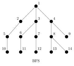 |
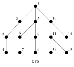 |
BFS first checks all of the children of the starting vertex, then all of their children, etc. It always completes a level before moving on to the next level. DFS works its way down the tree until it can't go any further then backs up to the first place where there is another route heading down that hasn't already been checked. It keeps this up until all routes have been checked.
We can extend these algorithms to graphs in general. We just need to keep a list of all the vertices that have previously been visited by the searching algorithm to prevent a cycle in the graph from causing an infinite loop.
Implementing BFS and DFS
First, we will consider a breadth first search that is given a starting vertex and returns a set consisting of all the vertices that can be reached from that vertex. The search relies on a relatively simple idea. We move through the graph and each time we find a new vertex we add it to a queue that keeps track of vertices that still need to be searched. We also maintain a set that keeps track of all the vertices we've been to. Here is the algorithm:
public static <T> Set<T> bfs(Graph<T> graph, T start)
{
Set<T> visited = new LinkedHashSet<T>();
Queue<T> queue = new ArrayDeque<T>();
visited.add(start);
queue.add(start);
while (!queue.isEmpty())
{
T v = queue.remove();
for (T u : graph.neighbors(v))
{
if (!visited.contains(u))
{
visited.add(u);
queue.add(u);
}
}
}
return visited;
}
Reading through it, we have written the method so that it takes a graph and a starting vertex as parameters. We being by adding the starting vertex to both the queue and the visited set. The queue holds the vertices we still have to visit. In the loop, we take the next thing off the queue and add all of its unvisited neighbors to the queue and the visited set. We keep looping until the queue is empty.
To implement DFS, all we have to do is change the queue to a stack, as below:
public static <T> Set<T> dfs(Graph<T> graph, T start)
{
Set<T> visited = new LinkedHashSet<T>();
Deque<T> stack = new ArrayDeque<T>();
visited.add(start);
stack.push(start);
while (!stack.isEmpty())
{
T v = stack.pop();
for (T u : graph.neighbors(v))
{
if (!visited.contains(u))
{
visited.add(u);
stack.push(u);
}
}
}
return visited;
}
With a queue, vertices were checked in the order they were added, which meant that since all the neighbors of a vertex were added at once, they would be checked one after another. With a stack, the next vertex to be checked is the most recently added vertex. So when we are checking a vertex and we add its children, its children put are higher in the stack than its siblings and so they are checked first. In short, BFS will always move to a brother or sister before checking a child, whereas DFS will do the opposite.
DFS can also be implemented relatively quickly using recursion. One of the exercises asks you to implement it.
BFS for finding a shortest path
BFS can be used to find the shortest path between two vertices in a graph. The main change we have to make is we use a map to keep track of the path. Each time we find a new vertex, we add an entry for it to the map, where the key is the vertex added and the value is its parent vertex, the vertex we were searching from when we found the vertex. Once we find our goal vertex, we will trace back through the map to get the path from the start to the goal vertex. Here is the code:
public static <T> List<T> bfsPath(Graph<T> graph, T start, T end)
{
Set<T> visited = new LinkedHashSet<T>();
Queue<T> queue = new ArrayDeque<T>();
Map<T, T> parent = new LinkedHashMap<T, T>();
visited.add(start);
queue.add(start);
parent.put(start, null);
while (!queue.isEmpty())
{
T v = queue.remove();
for (T u : graph.neighbors(v))
{
if (!visited.contains(u))
{
visited.add(u);
queue.add(u);
parent.put(u, v);
}
if (u.equals(end))
{
List<T> path = new ArrayList<T>();
while (u != null)
{
path.add(u);
u = parent.get(u);
}
Collections.reverse(path);
return path;
}
}
}
return new ArrayList<T>();
}
Replacing the queue with a stack would also find a path from the start to the goal vertex, but the resulting path may not be the shortest possible path. BFS is guaranteed to find the shortest path, while DFS often will find a path that is quite a bit longer. For instance, when I ran both of these searches on the word ladder graph from the previous section to find a word ladder from time to rise, BFS returned the ladder time → rime → rise, this being the shortest possible word ladder. DFS returned a list of 698 words, more than a third of the number of words in the list.
BFS vs DFS
Which search to use depends on the structure of the graph. If each vertex has a high degree, then since BFS searches every neighbor before moving on to the next level, BFS might take too long to find a solution that is several layers deep. However, if there are many possible end vertices, DFS might have a better chance of finding them. But in general, especially for small problems, DFS and BFS run quickly and the solution given by BFS will most be the most direction solution.
BFS and DFS are among the most straightforward searching algorithms and are the building blocks for more sophisticated searches. Do a web search or consult a textbook on algorithms for more.
Digraphs
A digraph is a graph in which the edges can be one-way (directed). The figure below shows a digraph.
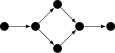
Digraphs model many real-life situations. For instance, a road network can be represented as a graph with the edges being roads and vertices being intersections or dead-ends. Directed edges could be used for one-way roads. Another example would be the graph of a game where the vertices are the states, with an edge between two vertices if it is possible to go between their corresponding states. In many games, once you make a move, you can't go back, so directed edges would be appropriate here.
We can build a digraph class by inheriting from our Graph class:
public class Digraph<T> extends Graph<T>
{
public void addEdge(T u, T v)
{
neighbors.get(u).add(v);
}
}
The only change is to the addEdge method. The addEdge method of the Graph class had an additional line neighbors.get(v).add(u), but since in a digraph edges go only one way, we don't want that line.
An application of digraphs
Here is an application of digraphs to a classic puzzle problem. Suppose we have two pails, one that holds 7 gallons and another that holds 11 gallons. We have a fountain of water where we can fill up and dump out our pails. Our goal is to get exactly 6 gallons just using these two pails. The rules are that you can only (1) fill up a pail to the top, (2) dump a pail completely out, or (3) dump the contents of one pail into another until the pail is empty or the other is full. There is no guestimating allowed.
For example, maybe we could start by filling up the 7-gallon pail, then dumping it into the 11-gallon pail. We could then fill up the 7-gallon pail and then dump it into the 11-gallon again, leaving 3 gallons in the 7-gallon pail. Maybe then we could dump the 11-gallon pail out completely. We could keep going doing operations like this until we have 6 gallons in one of the pails.
We can represent this problem with a digraph. The vertices are the possible states, represented as pairs (x,y), where x and y are the amount of water in the 7- and 11-gallon pails, respectively. There is an edge between two vertices if it is possible to go from their corresponding states, following the rules of the problem. For example, there is an edge between (3,0) and (0,0) because starting at the (3,0) state, we can dump out the 7-gallon pail to get to the (0,0) state. However, there is not an edge going in the opposite direction because there is no way to go from (0,0) to (3,0) in one step following the rules.
To create the graph, we first need a class to represent the states. The class has two integer fields, x and y. We have a simple toString method for the class and we override the equals method because we will need to test states for equality. We have used an IDE to generate that method. Though the code for this class is long, it is very simple and useful in other places.
public class Pair
{
public int x, y;
public Pair(int x, int y)
{
this.x = x;
this.y = y;
}
@Override
public String toString()
{
return "(" + x + ", " + y + ")";
}
@Override
public int hashCode()
{
final int prime = 31;
int result = 1;
result = prime * result + x;
result = prime * result + y;
return result;
}
@Override
public boolean equals(Object obj)
{
if (this == obj)
return true;
if (obj == null)
return false;
if (getClass() != obj.getClass())
return false;
Pair other = (Pair) obj;
if (x != other.x)
return false;
if (y != other.y)
return false;
return true;
}
}
The states for the problem are all pairs (x,y), where 0≤ x≤ 7 and 0≤ y≤ 11. Here is how we add those states to our digraph g:
for (int x=0; x<=7; x++)
for (int y=0; y<=11; y++)
g.add(new Pair(x,y));
To add the edges, we will loop over all vertices in the graph and add the appropriate edges for each. Here is the start of the loop:
for (Pair p : g)
{
int x=p.x, y=p.y;
g.addEdge(p, new Pair(x,0));
g.addEdge(p, new Pair(0,y));
g.addEdge(p, new Pair(x,11));
g.addEdge(p, new Pair(7,y));
// loop continues...
The four edges added above come from completely dumping out or completely filling one of the pails. There are other edges to add that come from dumping one of the pails into the other. These are a little trickier because there are a couple of cases to consider depending on whether the dumping completely empties or completely fills a pail. For instance, suppose we have 3 gallons in the 7-gallon pail. If there are 5 gallons in the 11-gallon pail, then (3,5) → (0,8) empties the 7-gallon pail, whereas if there are 9 gallons in the 11-gallon pail, then (3,9) → (1,11) completely fills the 11-gallon pail but doesn't empty the 7-gallon. We also have to avoid trying to pour into an already full pail or trying to pour from an empty pail. Here is the code that takes care of all of this:
// continuing the loop
if (x>0 && y<11)
{
if (x+y>11)
g.addEdge(p, new Pair(x-(11-y),11));
else
g.addEdge(p, new Pair(0, x+y));
}
if (y>0 && x<7)
{
if (x+y>7)
g.addEdge(p, new Pair(7,y-(7-x)));
else
g.addEdge(p, new Pair(x+y,0));
}
}
Once the digraph is complete, solving the puzzle boils down to using a BFS or DFS. Here is the complete class. Note that we use variables m and n in place of 7 and 11 so that the program will work with any size pails. The code assumes the bfsPath method is in a class called Searching.
WaterFountain wf = new WaterFountain();
Digraph<Pair> g = new Digraph<Pair>();
int m=7, n=11;
for (int x=0; x<=m; x++)
for (int y=0; y<=n; y++)
g.add(new Pair(x,y));
for (Pair p : g)
{
int x=p.x, y=p.y;
g.addEdge(p, new Pair(x,0));
g.addEdge(p, new Pair(0,y));
g.addEdge(p, new Pair(x,n));
g.addEdge(p, new Pair(m,y));
if (x>0 && y<n)
{
if (x+y>n)
g.addEdge(p, new Pair(x-(n-y),n));
else
g.addEdge(p, new Pair(0, x+y));
}
if (y>0 && x<m)
{
if (x+y>m)
g.addEdge(p, new Pair(m,y-(m-x)));
else
g.addEdge(p, new Pair(x+y,0));
}
}
System.out.println(Searching.bfsPath(g, new Pair(0,0), new Pair(6,0)));
When we run it, we get the following output:
[(0, 0), (7, 0), (0, 7), (7, 7), (3, 11), (3, 0), (0, 3), (7, 3), (0,10), (7, 10), (6, 11), (6, 0)]
This solution, given by BFS, is the most direct solution. DFS gives a longer solution:
[(0, 0), (7, 0), (0, 7), (7, 7), (3, 11), (7, 11), (0, 11), (7, 4), (0, 4), (4, 0), (4, 11), (7, 8), (0, 8), (7, 1), (0, 1), (1, 0), (1, 11), (7, 5), (0, 5), (5, 0), (5, 11), (7, 9), (0, 9), (7, 2), (0, 2), (2, 0), (2, 11), (7, 6), (0, 6), (6, 0)]
Weighted graphs
There is one more type of graph that we will consider, called a weighted graph. An example weighted graph is shown below. A weighted graph is like an ordinary graph except that the edges are given weights. We can think of edge weights as the cost of using edges.
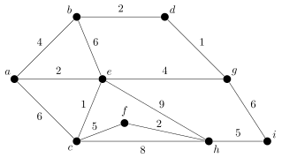
As an example, using a graph to model a network of cities, edge weights could represent the cost to get from one city to the other.
Our WeightedGraph class will be quite similar to our Graph class, with one big difference—how we represent edges. Since there are weights involved, we can't just use an adjacency list whose keys and values are both vertices. Instead, we will create an inner class called WeightedEdge and our adjacency list map will have keys that are vertices and values that are of type Edge. The Edge class will have fields for both endpoints and the weight. It will also have a toString method. For the application in the next section we will also need a method that returns a list of all the edges in the graph, so we will add that into our class. Here is everything:
import java.util.ArrayList;
import java.util.Iterator;
import java.util.LinkedHashMap;
import java.util.List;
import java.util.Map;
public class WeightedGraph<T> implements Iterable<T>
{
public static class Edge<U>
{
public U v1;
public U v2;
public int weight;
public Edge(U v1, U v2, int weight)
{
this.v1 = v1;
this.v2 = v2;
this.weight = weight;
}
@Override
public String toString()
{
return "(" + v1 + ", " + v2 + ", " + weight + ")";
}
}
private Map<T, List<Edge<T>>> neighbors;
private List<Edge<T>> edges;
public WeightedGraph()
{
neighbors = new LinkedHashMap<T, List<Edge<T>>>();
edges = new ArrayList<Edge<T>>();
}
public void add(T v)
{
if (!neighbors.containsKey(v))
neighbors.put(v, new ArrayList<Edge<T>>());
}
public void addEdge(T u, T v, int weight)
{
neighbors.get(u).add(new Edge<T>(u, v, weight));
neighbors.get(v).add(new Edge<T>(v, u, weight));
edges.add(new Edge<T>(u, v, weight));
}
public List<T> neighbors(T u)
{
List<T> nbrs = new ArrayList<T>();
for (Edge<T> e : neighbors.get(u))
nbrs.add(e.v2);
return nbrs;
}
public List<Edge<T>> getEdges()
{
return new ArrayList<Edge<T>>(edges);
}
@Override
public Iterator<T> iterator()
{
return neighbors.keySet().iterator();
}
}
Kruskal's algorithm for minimum spanning trees
One thing people are interested in about weighted graphs is finding a minimum spanning tree. A spanning tree of a weighted graph is a subgraph of the graph that includes all the vertices and has no cycles. A minimum spanning tree is a spanning tree where the sum of the weights of the edges in the tree is as small as possible. A minimum spanning tree is highlighted in the graph below.
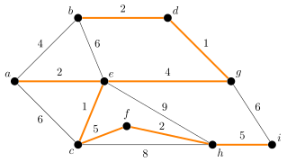
One way to think of this is that the vertices are cities, the edges are potential roads, and the weights are the costs of building the roads. Say we want to connect all the cities so that it is possible to travel along the network from any city to any other. A minimum spanning tree will give the cheapest way of doing this. The “spanning” part means it includes every city, and the “tree” part means that there are no cycles. Having a cycle would mean there were two ways of getting from a certain city to another, and you could remove one of them to get a cheaper road network without disconnecting the cities.
There are two common algorithms for finding minimum spanning trees. The one we will look at is Kruskal's algorithm (the other is called Prim's algorithm). It is a surprising algorithm in that it you do just about the simplest thing you can think of and it ends up giving the optimal answer. At each step in the algorithm, pick the remaining edge that has the smallest weight (breaking ties arbitrarily) and add it to the tree, provided adding it doesn't create a cycle. We don't want cycles because trees cannot have cycles, and thinking in terms of the road network, having a cycle would mean we have a redundant edge.
In the graph above, we would start by adding edges ce and dg of weight 1. We then add edges bd, ae, and fh, each of weight 2. Then we add edge eg of weight 4. We don't add edge ab of weight 4 because that would create a cycle. Alternatively, we could have added ab and not eg. Either way would work. There are often several spanning trees of the same total weight. Finally, we add edges ci and hi to get a minimum spanning tree of total weight 22. No other spanning tree has a smaller weight.
To implement this algorithm, we have two things to do. First, we have to order the edges by weight. One way to do this would have be to store the edges in a data structure like a TreeSet or a BST as we added them. A bit slower, but easier approach is to make the list from the keys of the edge map and then sort the resulting list. The trick is that we have to sort the edges by their weights. To do this, we use Collections.sort in a special way. See this section for more on this topic.
The other thing we need to do to implement the algorithm is to make sure that adding an edge does not create a cycle. This can be a little tricky. One clever way to do this is as follows: Create a list of sets, one for each vertex in the graph. Then each time we add an edge to the tree, we
merge the sets corresponding to the endpoints of the edge. For example, in the graph shown earlier, the list of sets will change as follows:
| Added edge | List of sets |
|---|---|
| -- | [{a}, {b}, {c}, {d}, {e}, {f}, {g}, {h}, {i}] |
| dg | [{a}, {b}, {c}, {d,g}, {e}, {f}, {h}, {i}] |
| ce | [{a}, {b}, {c,e}, {d,g}, {f}, {h}, {i}] |
| bd | [{a}, {b,d,g}, {c,e}, {f}, {h}, {i}] |
| ae | [{a,c,e}, {b,d,g}, {f}, {h}, {i}] |
| fh | [{a,c,e}, {b,d,g}, {f,h}, {i}] |
| eg | [{a,b,c,d,e,g}, {f,h}, {i}] |
| eg | [{a,b,c,d,e,g}, {f,h}, {i}] |
| cf | [{a,b,c,d,e,f,g,h}, {i}] |
| hi | [{a,b,c,d,e,f,g,h,i}] |
The idea is that the sets stand for the connected regions of the soon-to-be tree. Initially, it is completely disconnected, with all the vertices disconnected from each other. We then add edge dg, which connects d and g, and we now have the set {d,g} in the list, representing that d and g are now connected to each other. Two steps later, we add the edge bd, which connects b to d, and therefore to g, and so we end up with the set {b,d,g} in the list. We now have a region where b, d, and g are connected to each other. The process continues until there is only one set in the list, meaning that all the vertices have been connected.
To check to see if adding an edge creates a cycle, we just have to check to see if the start and endpoints are in the same set. If they are, then they are already connected and so we don't want to add that edge. If they are not in the same set, then we merge the sets corresponding to the two endpoints of the edge to indicate that now everything connected to the one endpoint and everything connected to the other are now all connected together. The code for the algorithm is shown below.
public static <T> List<WeightedGraph.Edge<T>> kruskal(WeightedGraph<T> graph)
{
List<WeightedGraph.Edge<T>> mstEdges = new ArrayList<WeightedGraph.Edge<T>>();
List<WeightedGraph.Edge<T>> edges = graph.getEdges();
Collections.sort(edges, (s,t) -> s.weight - t.weight); // Requires Java 8 or later
List<Set<T>> sets = new ArrayList<Set<T>>();
for (T v : graph)
sets.add(new LinkedHashSet<T>(Collections.singleton(v)));
while (sets.size() > 1 && edges.size() != 0)
{
WeightedGraph.Edge<T> edge = edges.remove(0);
int setIndex1=0, setIndex2=0;
for (int i=0; i<sets.size(); i++)
{
if (sets.get(i).contains(edge.v1))
setIndex1 = i;
if (sets.get(i).contains(edge.v2))
setIndex2 = i;
}
if (setIndex1 != setIndex2)
{
sets.get(setIndex1).addAll(sets.get(setIndex2));
sets.remove(setIndex2);
mstEdges.add(edge);
}
}
if (edges.size() == 0)
return new ArrayList<WeightedGraph.Edge<T>>();
else
return mstEdges;
}
Here is a little code to test it out on the graph from the beginning of the section:
WeightedGraph<String> g = new WeightedGraph<String>();
String v = "abcdefgh";
for (int i=0; i<v.length(); i++)
g.add(v.substring(i,i+1));
String e = "a b 4, a e 2, a c 6, b d 2, b e 6, c e 1, c f 5, c h 8,
d g 1, e g 4, f h 2, g i 6, h i 5"
for (String x : e.split(", "))
{
String[] a = x.split(" ");
g.addEdge(a[0], a[1], Integer.parseInt(a[2]));
}
System.out.println(kruskal(g));
Kruskal's algorithm is called a greedy algorithm because at each step you choose the minimum edge available. In general, greedy algorithms work such that at each step you always take the least-cost or most-cost move.
Exercises
- For the graph below, show both its adjacency matrix representation and its adjacency list representation.
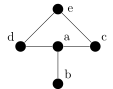
- Add the following methods to the
Graphclass.-
size()— returns the number of vertices in the graph. -
numberOfEdges()— returns how many edges are in the graph. -
isEmpty()— returns whether or not there are any vertices in the graph. -
degree(v)— returns how many neighbors vertexvhas. -
contains(v)— returns whether or notvis a vertex in the graph. -
containsEdge(u,v)— returns whether or not there is an edge betweenuandv. -
remove(v)— removes vertexvfrom the graph. -
removeEdge(u,v)— removes the edge betweenuandvfrom the graph. -
toString— returns a string representation of the graph, with each line consisting of a vertex name, followed by a colon, followed by the vertex's neighbors, with a space between each neighbor. For instance, if the graph consists of vertices a, b, c, d, and e with edges ab, ac, and cd, the string should look like the following:a : b c b : a c : b d d : c e : -
distance(u,v)— returns the distance between two vertices. The distance is the length of the shortest path between the vertices. -
isConnectedTo(u, v)— returnstrueif it is possible to get from vertexuto vertexvby following edges. -
isConnected()— returnstrueif the graph is connected andfalseotherwise. A graph is connected if it is possible to get from any vertex to any other vertex. -
findComponent(v)— returns a list of all the vertices that can be reached from vertexv -
components(v)— returns a list of all the components of a graph. A component in a graph is a collection of vertices and edges in the graph such that it is possible to get from any vertex to any other vertex in the component. -
isCutVertex(v)— returnstrueifvis a cut vertex, a vertex whose deletion disconnects the graph. -
isHamiltonianCycle(a)— returnstrueif the list of verticesarepresent a Hamiltonian cycle. A Hamiltonian cycle is a cycle that includes every vertex. -
isValidColoring(m)— returnstrueif the mapmrepresents a valid coloring of the graph andfalseotherwise. A coloring of a graph is an assignment of colors to the vertices of the graph such that adjacent vertices are not given the same color. The argumentmis a map whose keys are the vertices of the graph and whose values are the colors (integers) assigned to the vertices. Usually positive integers are used for the color names. -
findValidColoring()— returns a map like in the previous problem that represents a valid coloring of the graph. Create the map using the following greedy algorithm: Loop through the vertices in any order, assign each vertex the smallest color (starting with the number 1) that has not already been assign to one of its neighbors. -
isEulerian()— returnstrueif the graph is Eulerian and false otherwise. A graph is Eulerian if one can traverse the graph using every edge exactly once and end up back at the starting vertex. A nice theorem says that a graph is Eulerian if and only if every vertex has even degree. -
inducedSubgraph(list)— given a list of vertices, returns a new graph object which consists of the vertices in the list and all the edges in the original graph between those vertices.
-
- Add the methods from the previous problem to the
AGraphclass that uses an adjacency matrix. - In a file separate from the
Graphclass, create the following methods:-
addAll(g, s)— Assuminggis a graph whose vertices are strings andsis a string with vertex names separated by spaces, this method adds vertices togfor each vertex name ins. For instance, ifs = "a b c d", this method will add vertices nameda,b,c, anddto the graph. Vertex names may be more than one character long. -
addEdges(g, s)— Assuminggis a graph whose vertices are strings andsis a string of edges separated by spaces, this method adds edges togfor each edge name ins. Each edge is in the formendpoint1-endpoint2. For instance, ifs = "a-b a-c b-c", this method will add edges fromatob, fromatoc, and frombtoc. Vertex names may be more than one character long.
-
- Add methods called
indegreeandoutdegreeto theDigraphclass. The indegree of a vertex is the number of edges directed into it, and the outdegree of a vertex is the number of edges directed out from it. - For the graphs below, we are starting at vertex a. Indicate the order in which both breadth-first search and depth-first search visit the vertices.
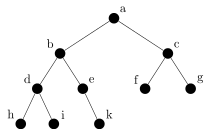
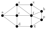
- Here is a puzzle that is at least 1200 years old: A traveler has to get a wolf, a goat, and a cabbage across a river. The problem is that the wolf can't be left alone with the goat, the goat can't be left alone with the cabbage, and the boat can only hold the traveler and a single animal/cabbage at once. How can the traveler get all three items safely across the river? Solve this problem by representing it with a graph and using a breadth-first search to find a solution.
- The Internet Movie Database (IMDB) provides text files containing info on which actors and actresses were in which movies. One such file consists of thousands of lines, one line per movie. Each line starts with the title of the movie and is followed by a list of the people that acted in the movie. Each entry (including the title) is separated from the other entries by a slash, /. Read through the text file and put the information into a graph (you will have to decide how to structure the graph). Then prompt the user for the names of two actors and output the shortest path of the form (actor → movie → actor → movie → … → actor) that runs between the two actors. For instance, here is the shortest path between Meryl Streep and Sly Stallone:
[Streep, Meryl, Adaptation. (2002), Beaver, Jim (I), Nighthawks (1981), Stallone, Sylvester]
- Modify the depth-first search and breadth-first search methods so that instead of a single goal vertex as a parameter, they receive a list of goal vertices as a parameter. The search is successful if any of the vertices in the list are found.
- Write a recursive version of the depth first search algorithm.
- In this chapter we created a digraph class and a weighted graph class. Combine the ideas used in those classes to created a weighted digraph class.
- Find a minimum spanning tree in the graph below. Please shade its edges on the graph and also give the total weight of your spanning tree. Also, show the sets used by Kruskal's algorithm at each step.
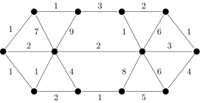
- The table below gives the cost of building a road between various cities. An entry of ∞ indicates that the road cannot be built. The goal is to find the minimum cost of a network of roads such that it is possible to get from any city to any other. This problem can be solved with Kruskal's algorithm. Set up the graph in Java and use the method we wrote in this section to find the solution.
a b c d e a 0 3 5 11 9 b 3 0 3 9 8 c 5 3 0 ∞ 10 d 11 9 ∞ 0 7 e 9 8 10 7 0 - Modify the depth-first search algorithm to create a function
hasCycle(g)that determines ifthe graph
ghas a cycle. [Hint: if depth-first search encounters a vertex that it has already seen, thatindicates that there is a cycle in the graph. Just be careful that that vertex doesn't happen to be the
parent of the vertex currently being checked.]
- Modify the depth-first search algorithm from class to create a function
isBipartite(g)thatdetermines if the graph
gis bipartite. A graph is bipartite if its vertices can be partitioned into two setssuch that the only edges in the graph are between the two sets, with no edges within either set. One
way to approach this problem is to label each vertex as you visit it with a 0 or 1. Labels should
alternate so that all the neighbors of a vertex v should have the opposite label of what v has. If there is
ever a conflict, where a vertex is already labeled and this rule would try to assign it a different label,
then the graph is not bipartite.
- Consider the puzzle problem below. Find a way to represent it as a graph, program that implementation, and run breadth-first search on it to find a solution.
Five professors and their five dogs were having a lot of fun camping. Each professor owned one of the dogs. While they were all on a hike, they came to a river they had to cross. There was a small motorboat alongside the river. They determined that the boat was only large enough to hold three living things—either dogs or professors. Unfortunately, the dogs were a little temperamental, and they really didn't like the professors. Each dog was comfortable with its owner and no other professor. Each dog could not be left with the professors unless the dog's owner was present—not even momentarily! Dogs could be left with other dogs, however. The crossing would have been impossible except Professor A's dog, which was very smart, knew how to operate the boat. None of the other dogs were that smart, however. How was the crossing arranged, and how many trips did it take?
Sorting
This chapter is about a variety of different algorithms for sorting arrays and lists. Most higher level languages have sorting built in to the language (for instance, Java has Collections.sort and Arrays.sort), so it not as useful now to know how to sort things as it once was, when programmers often had to implement their own sorts. However, it is still useful to know how some of the different sorts work. It is also good practice to implement the algorithms. Knowledge of these things is considered foundational computer science knowledge, and moreover, some of the ideas behind the algorithms are useful in other situations. A few notes:
- We will implement all the searches on integer arrays instead of on generic lists. The reason for this is that array syntax is simpler and more readable than list syntax. In practice, though, it is usually better to use lists in place of arrays. It is not hard to translate the array algorithms to list algorithms. This is covered in this section.
- For clarity, the figures demonstrating the sorts will use letters instead of numbers.
- Our sorts will directly modify the caller's array. We could also leave the array untouched and return a new sorted array, but we've chosen this approach for simplicity.
Selection Sort
Selection Sort is one of this simplest sorts to implement, but it is also slow. It works as follows:
Start by considering the first element of the array versus all the other elements. Find the smallest element among the others and if it is less than the first element, then swap them. Now move on to the second element of the array. Look at all the elements after the second, find the smallest element among them, and if it is smaller than the second element, then swap them. Then we move on to the third element of the array. Look at all the elements after it, find the smallest among them, and if it is smaller than the third element, then swap it with the third element. Continue this process, moving one element forward, until you reach the end of the array.
The way it works is shown in the figure below. At each stage, the left of the two highlighted letters is the position that is being worked on and the right highlighted letter is the minimum of the remaining letters. Those two are swapped if the right one is smaller. Notice how the array gets sorted from left to right.
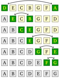
To implement it, we use nested loops. The outer loop is for the position that is being worked on. The inner loop finds the minimum of the remaining elements. Here is the code:
public static void selectionSort(int[] a)
{
for (int i=0; i<a.length-1; i++)
{
int smallest = i;
for (int j=i+1; j<a.length; j++)
if (a[j] < a[smallest])
smallest = j;
int hold = a[i];
a[i] = a[smallest];
a[smallest] = hold;
}
}
This is an O(n2) algorithm. The outer loop that runs n-1 times, while the inner loop averages out to running n/2 times. This gives a total of n(n-1)/2 comparisons. The algorithm always makes this number of comparisons, no matter if the array is already sorted or completely jumbled.
Selection Sort is one of the slowest sorts around, but is very quick to code. In fact, for simplicity of coding, here is a variant of Selection Sort that is especially quick to code. It just contains two loops, a comparison, and a swap statement:
public static void selectionSortVariant(int[] a)
{
for (int i=0; i<a.length-1; i++)
{
for (int j=i+1; j<a.length; j++)
{
if (a[i]>a[j])
{
int hold = a[i];
a[i] = a[j];
a[j] = hold;
}
}
}
}
Bubble Sort
Bubble Sort is a relative of Selection Sort. We start at the end of the array and compare the last and second-to-last elements, swapping if necessary. We then compare the second-to-last element with the third-to-last. Then we compare the third-to-last with the fourth-to-last. We keep going in this way until we reach the front of the array. At this point, the first position in the array will be correct. The correct element “bubbles up” to the front of the array. We then start at the end of the array and repeat the process, but this time instead of going all the way to the front, we stop at the second element (because we know the first element is already correct). After this stage, the second element is correct.
We then continue the process, where at each step, we start at the end of the array and compare adjacent elements and continue doing that until we get to the stopping point. At each step, the stopping point moves one index forward until we reach the end of the array. The figure below shows the order in which elements are compared. The arrows indicate when a swap is performed.
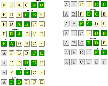
We use nested for loops to implement the algorithm. The outer loop keeps track of the stopping point. It starts at the front of the array and works its way toward the end. The inner loop always starts at the end of the array and ends at the stopping point. Inside the loop we compare adjacent elements and swap if necessary.
public static void bubbleSort(int[] a)
{
for (int i=0; i<a.length-1; i++)
{
for(int j=a.length-1; j>i; j--)
{
if (a[j-1] > a[j])
{
int hold = a[j-1];
a[j-1] = a[j];
a[j] = hold;
}
}
}
}
Just like Selection Sort, Bubble Sort is O(n2), making n(n-1)/2 comparisons, regardless of whether the array is already sorted or completely jumbled. However, we can actually improve on this. If there are no swaps made on one of the passes through the array (i.e., one run of the inner loop), then the array must be sorted and we can stop. One of the exercises is about implementing this. This improvement, however, is still not enough to make the Bubble Sort useful for sorting large arrays. In fact, its performance can be worse than the ordinary Bubble Sort for large, well-mixed arrays. Because of its slow performance, Bubble Sort is rarely used, but it is simple and one of the most well-known sorting algorithms.
Insertion Sort
Insertion sort is the last and the fastest of the O(n2) sorting algorithms we will look at. Here is how it works:
Say we have a stack of papers we want to put into in alphabetical order. We could start by putting the first two papers in order. Then we could put the third paper where it fits in order with the other two. Then we could put the fourth paper where it fits in order with the first three. If we keep doing this, we have what is essentially Insertion Sort.
To do Insertion Sort on an array, we loop over the indices of the array running from 1 to the end of the array. For each index, we take the element at that index and loop back through the array towards the front, looking for where the element belongs among the earlier elements. These elements are in sorted order (having been placed in order by the previous steps), so to find the location we run the loop until we find an element that is smaller than the one we or looking at or fall off the front of the array. The figure below shows it in action.
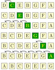
Here is the code:
public static void insertionSort(int[] a)
{
for (int i=1; i<a.length; i++)
{
int hold = a[i];
int j = i;
while (j>=1 && a[j-1]>hold)
{
a[j] = a[j-1];
j--;
}
a[j] = hold;
}
}
With the outer for loop we look at a new element at each time. The inner while loop looks for the right place to put that element. Notice that, unlike Bubble Sort and Selection Sort, there is no need to swap elements. Instead, we can use a[j] = a[j-1] to move things down the line and then a[j] = hold to finish.
Insertion Sort is faster than both Selection Sort and Bubble Sort, but it is still an O(n2) algorithm. Insertion Sort will usually make less comparisons than the other two, but we still have nested loops and on average, the number of comparisons needed is still quadratic and hence unsuitable for sorting large arrays. However, for small arrays it is very fast, faster in fact than just about anything else including the O(n log n) algorithms in the upcoming sections. The key is that those algorithms require a certain amount of setup work or overhead due to recursion that Insertion Sort doesn't. Once they get going, however, they will usually outperform Insertion Sort.
If the list is already sorted, the condition on the inner while loop will always be false and Insertion Sort runs in O(n) time, which is the best any sorting algorithm can manage. In fact, Insertion Sort can run relatively quickly even on very large arrays if those arrays are nearly sorted. On the other hand, if the list is in reverse order, the while loop condition is always true and we have n(n-1)/2 swaps, just as bad as Selection Sort and Bubble Sort.
Shellsort
Shellsort builds on Insertion Sort. Here is an example of one variation of Shellsort. We start by pulling out every fourth character starting with the first, and using Insertion Sort to sort just those characters. We then pull out every fourth character starting with the second character, and use Insertion Sort to sort those characters. We do the same for every fourth character starting with the third and then every fourth starting with the fourth. See the figure below:
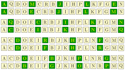
At this point the array is nearly sorted.
We run a final insertion sort on the entire array to sort it. This step is pretty quick because only a few swaps need to be made before the array is sorted. Now it may seem like we did so many individual sorts that it would have been more efficient to just have run a single insertion sort in the first place, but that is not the case. The total number of comparisons and swaps needed will often be quite a bit less for Shellsort than for Insertion Sort.
In the example above, we used gaps of length 4, 2, and 1. The sequence (4,2,1) is called a gap-sequence. There are a variety of different gap sequences one could use, the only requirement being that the last gap is 1. An implementation of Shellsort is shown below using a very specific gap sequence. The code is surprisingly short and very efficient as it essentially works on all the subarrays for a given gap at once. In the example above, with a gap of 4, we did four separate steps, but the code below would handle them all together.
public static void shellsort(int[] a)
{
int[] gaps = {1391376, 463792, 198768, 86961, 33936, 13776, 4592,
1968, 861, 336, 112, 48, 21, 7, 3, 1};
for (int gap : gaps)
{
for (int i=gap; i<a.length; i++)
{
int hold = a[i];
int j = i;
while (j>=gap && a[j-gap]>hold)
{
a[j] = a[j-gap];
j-=gap;
}
a[j] = hold;
}
}
}
Different gap sequences produce different running times. Some produce an O(n2) running time, while others can get somewhat closer to O(n), with running times like O(n5/4) or O(n3/2). Determining the running time for a given gap sequence can be tricky. In fact, the running times for some popular gap sequences are unknown. People are even now still looking for better gap sequences. Shellsort is not quite as popular as the sorts coming up in the next few sections, but it is a nice sort with performance comparable to those algorithms in a few specific applications.
Heapsort
Heapsort uses a heap to sort an array. Recall that a heap is a data structure that gives easy access to the smallest item in a collection. Using a heap to sort an array is very easy—we just run through the array, putting the elements one-by-one onto the heap and when that's done, we then one-by-one remove the top (minimum) element from the heap.
The PriorityQueue class in Java's Collections Framework is implemented using a heap. So we can use Java's PriorityQueue to implement Heapsort. Here is the code:
public static void heapsort(int[] a)
{
PriorityQueue<Integer> heap = new PriorityQueue<Integer>();
for (int i=0; i<a.length; i++)
heap.add(a[i]);
for (int i=0; i<a.length; i++)
a[i] = heap.remove();
}
Heapsort has an O(n log n) running time. When we insert the elements into the heap we have to loop through the array, so that's where the n comes from. Adding each element to the heap is an O(log n) operation, so overall adding the elements of the array into the heap takes O(n log n) time. Removing them also takes O(n log n) time. Heapsort is one of the faster sorts. It runs in O(n log n) time regardless of whether the data is already sorted, in reverse order, or whatever.
A close relative of Heapsort is Treesort that works in the same way but uses a BST in place of a heap. One of the exercises asks you to implement it.
Merge Sort
Merge Sort works as follows: We break the array into two halves, sort them, and then merge them together. The halves themselves are sorted with Merge Sort, making this is a recursive algorithm. For instance, say we want to sort the string CEIGJBFDHA. We break it up into two halves, CEIGJ and BFDHA. We then sort those halves (using Merge Sort) to get CEGIJ and ABDFH and merge the sorted halves back together to get ABCDEFGHIJ. See the figure below:
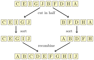
We will break up the work into sorting and merging. Here is the sorting code:
public static void mergeSort(int[] a)
{
if (a.length <= 1)
return;
int[] left = Arrays.copyOfRange(a, 0, a.length/2);
int[] right = Arrays.copyOfRange(a, a.length/2, a.length);
mergeSort(left);
mergeSort(right);
int[] m = merge(left, right);
for (int i=0; i<a.length; i++)
a[i] = m[i];
}
The base case of the recursion is a list of size 0 or 1, which doesn't require any sorting. To find the left and right halves of the array, we use the copyOfRange method from java.util.Arrays. We then call mergeSort on each, merge the two sorted halves, and copy the result back into a.
Here is the merging code. The way it works is we maintain counters to keep track of where we are in the left and right arrays. We loop through, looking at the elements at the current location in each array, adding the smaller of the two to the merged array and then updating the appropriate counter. We stop when we reach the end of either array. At this point, there still may be some elements left over in the other array, so we add all of them to the merged array.
private static int[] merge(int[] left, int[] right)
{
int[] mergedArray = new int[left.length + right.length];
int x=0, y=0, z=0;
while (x < left.length && y < right.length)
{
if (left[x]<right[y])
mergedArray[z++] = left[x++];
else
mergedArray[z++] = right[y++];
}
if (x < left.length)
{
for (int i=x; i<left.length; i++)
mergedArray[z++] = left[i];
}
else if (y < right.length)
{
for (int i=y; i<right.length; i++)
mergedArray[z++] = right[i];
}
return mergedArray;
}
One thing to note is that to keep the code short, we use the ++ operator. When used like this, the incrementing happens after the assignment. So, for instance, the code on the left is equivalent to the code on the right.
if (left[x] < right[y]) if (left[x] < right[y])
mergedArray[z++] = left[x++]; {
mergedArray[z] = left[x];
z++;
x++;
}
This version of Merge Sort is a little slow. There are several places that it can be improved, but one in particular stands out—we waste a lot of time creating new arrays. There is a way around this where we will do most of the sorting and merging within the original array. We will need to create just one other array, b, with the same size as a as a place to temporarily store some things when merging. The key is that instead of creating the left and right arrays, we will work completely within a, using indices called left, mid, right to keep track of where in the array we are currently sorting. These become parameters to the merge function itself. The faster code is below:
public static void mergeSort(int[] a)
{
int[] b = new int[a.length];
mergeSortHelper(a, b, 0, a.length);
}
private static void mergeSortHelper(int[] a, int[] b, int left, int right)
{
// base case
if (right-left <= 1)
return;
// recursive part
int mid = (left + right) / 2;
mergeSortHelper(a, b, left, mid);
mergeSortHelper(a, b, mid, right);
// merging
for (int i=left; i<right; i++)
b[i] = a[i];
int x=left, y=mid, z=left;
while (x<mid && y<right)
{
if (b[x] < b[y])
a[z++] = b[x++];
else
a[z++] = b[y++];
}
if (x < mid)
{
for (int i=x; i<mid; i++)
a[z++] = b[i];
}
else if (y < right)
{
for (int i=y; i<right; i++)
a[z++] = b[i];
}
}
Merge Sort has an O(n log n) running time for all input arrays. Intuitively, the logarithm comes from the fact that we are cutting things in half at each step. The n comes from the fact that the merging algorithm is O(n).
Because of the overhead involved in recursion, Merge Sort can be outperformed by Insertion sort for small arrays. This suggests a way to speed Merge Sort up a little. Instead of our current base case taking effect at length 0 or 1, for small arrays we call Insertion Sort, like below:
if (a.length <= 100)
insertionSort(a);
Merge Sort is fast. The sort method built in to Python is a variant of Merge Sort called Timsort. Java 7 and 8 also use Merge Sort and Timsort in addition to a variant of Quicksort.
Quicksort
Quicksort, like Merge Sort, is a sort that works by breaking the array into two subarrays, sorting them and then recombining. The figure below shows how it works.
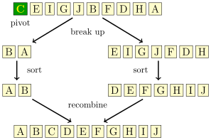
One subarray, called smaller, consists of all the elements less than the first element in the array and the other subarray, called larger, consists of all the elements greater than or equal to it. For instance, if we are sorting CEIGJBFDHA, the subarray smaller is BA (everything less than the first element, C) and the subarray larger is EIGJFDH (everything greater than C). We do this by scanning through the array and putting all the elements that are less than the first element (called the pivot) into smaller and putting the rest into larger.
We then sort the two subarrays using Quicksort again, making this a recursive algorithm. Finally, we combine the subarrays. Because we know that all the things in smaller are less than the pivot and all the things in larger are greater than or equal to the pivot, we build our sorted array by adding the elements of smaller (which are now sorted), then adding the pivot, and then adding the elements of larger.
Notice that the way Quicksort breaks up the array is more complicated way than the way Merge Sort does, but then Quicksort has an easier time putting things back together than Merge Sort does. Here is the Quicksort code:
public static void quicksort(int[] a)
{
if (a.length <= 1)
return;
int[] smaller = new int[a.length-1];
int[] larger = new int[a.length-1];
int pivot = a[0];
// build the subarrays
int d = 0, e = 0;
for (int i=1; i<a.length; i++)
{
if (a[i]<pivot)
smaller[d++] = a[i];
else
larger[e++] = a[i];
}
smaller = Arrays.copyOf(smaller, d);
larger = Arrays.copyOf(larger, e);
// recursive part
quicksort(smaller);
quicksort(larger);
// put back together
int c = 0;
for (int x : smaller)
a[c++] = x;
a[c++] = pivot;
for (int x : larger)
a[c++] = x;
}
There is a problem with our implementation—contrary to its name, our algorithm is slow. Creating the subarrays is very time-consuming, particularly because we create two new arrays, recopy them, and then put them back together. We can get a considerable speedup by doing the partition in-place. That is, we will not create any new arrays, but instead we will move things around in the main array. This is not unlike how we sped up our Merge Sort implementation. The process is shown in the figure below:
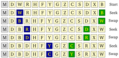
We have two indices, i and j, with i starting at the left end of the array and j starting at the right. Both indices will move towards the middle of the array. We first advance i until we meet an element that is greater than or equal to the pivot. We then advance j until we meet an element that is less than or equal to the pivot. When this happens, we swap the elements at each index. We then continue advancing the indices and swapping in the same way, stopping the process once the i and j indices pass by each other.
In the figure above, the pivot is M, the first letter in the array. The figure is broken down into “seek” phases, where we advance i and j, and swap phases. The blue highlighted letter on the left corresponds to the position of i and the green highlighted letter on the right corresponds to the position of j. Notice at the last step how they cross paths.
This process partitions the array. We then make recursive calls to Quicksort, using the positions of the indices i and j to indicate where the two subarrays are located in the main array. In particular, we make a recursive call on the subarray starting at the left end and ending at the position of i, and we make a recursive call on the subarray starting at the position of j and ending at the right end. So in the example above, we would call Quicksort on the subarrays from 0 to 6 and from 7 to 11.
Here is the code for our improved Quicksort:
public static void quicksort(int[] a)
{
quicksort_helper(a, 0, a.length-1);
}
public static void quicksort_helper(int[] a, int left, int right)
{
if (left >= right)
return;
int i=left, j=right, pivot=a[left];
while (i <= j)
{
while (a[i] < pivot)
i++;
while (a[j] > pivot)
j--;
if (i <= j)
{
int hold = a[i];
a[i] = a[j];
a[j] = hold;
i++;
j--;
}
}
quicksort_helper(a, i, right);
quicksort_helper(a, left, j);
}
Notice that because we are using the same array for everything, we need to have two additional parameters to the Quicksort function, left and right, which indicate which part of the array we are currently working on. There are a few subtleties here that we will skip over. Namely, it isn't obvious that the two inner while loops will always terminate. Also, it is possible for values equal to the pivot to end up in either the left or right halves after any partition, but in the end, this will work out. This approach gives a big improvement in speed.
Quicksort generally has an O(n log n) running time, but there are some special cases where it degenerates to O(n2). One of these would be if the array was already sorted. In that case the subarray smaller will be empty, while the subarray larger will have size n-1. When we call Quicksort on larger, we will again have the same problem, so we will end up with n total recursive calls. Since real-life arrays are often sorted or nearly so, this is an important problem. One way around this problem is to use a different pivot, such as one in the middle of the array.
Quicksort is one of the fastest sorting algorithms around. It is built into a number of programming languages.
Counting Sort
If we know something about the data in our array, then we can do better than the O(n log n) algorithms we've seen in the last few sections. For instance, if we know that we know the array contains only values in a relatively small range, then we can use an O(n) sort known as Counting Sort.
Counting Sort works by keeping an array of counts of how many times each element occurs in the array. We scan through the array and each time we meet an element, we add 1 to its count. So for instance, suppose we know that our arrays will only contain integers between 0 and 9. If we have the array [1,2,5,0,1,5,1,3,5], the array of counts would be [1,3,1,1,0,3,0,0,0,0] because there is 1 zero, 3 ones, 1 two, 1 three, no fours, 3 fives, and no sixes, sevens, eights, or nines.
We can then use this array of counts to construct the sorted list [0,1,1,1,2,3,5,5,5] by repeating 0 one time, repeating 1 three times, repeating 2 one time, etc., starting from 0 and repeating each element according to its count. Here is the Counting Sort algorithm implemented for arrays with values between 0 and 99:
public static void countingSort(int[] a)
{
int[] counts = new int[100];
for (int x : a)
counts[x]++;
int c=0;
for (int i=0; i<counts.length; i++)
for (int j=0; j<counts[i]; j++)
a[c++] = i;
}
This simple sort has an O(n) running time. The only drawback is that it only works if the array consists of integers between 0 and 99. We can change the size of the counts array to something larger, like 10,000 or 100,000 to get it to work with arrays that contain larger numbers, but this approach becomes infeasible if the array could contain very large integers.
Comparison of sorting algorithms
First, Merge Sort and Quicksort are considered to be the fastest sorts. Insertion Sort can be better than those on small arrays (of size around 10 to 100, depending on a variety of factors). Heapsort is competitive with Merge Sort and Quicksort, but is not quite as fast. Shellsort can be competitive with these sorts in a few specific applications. Selection Sort and Bubble Sort are mostly of historical interest.
In terms of asymptotics, the running time of a sort must always be at least O(n) because you have to look at every element before you know if the array is sorted. We have seen that Counting Sort achieves the O(n) optimum, but it is limited in where it can be used. Also, it can be shown that any sort that works by comparing one element to another must have a running time of at least O(nlog n). The O(n log n) sorts that we have seen are Heapsort, Merge Sort, and Quicksort.
Regarding the big O running times, remember that there are constants involved. For instance, Selection Sort and Bubble Sort are both O(n2) algorithms, but it may turn out that Selection Sort's running time is something like 10n2 and Bubble Sort's is 15n2, making Selection a bit faster. Or a bit more practically, the O(n2) Insertion Sort beats the O(n log n) Merge Sort for small arrays. This could happen if Insertion Sort's running time looks like 0.2n2 and Merge Sort's running time looks like 2n log n. For values up until around 50, 0.2n2 is smaller, but then the n2 term starts to dominate n log n and 2n log n ends up better for larger values.
There is more to the story than just big O. One thing that matters is exactly how the algorithms are implemented and on what sort of data they will be used. For instance, working with integer arrays where comparisons are simple is a lot different than working on arrays of objects where the comparison operation might be fairly complex. Another consideration is memory usage. Most of the O(n log n) algorithms have memory usage associated with either a data structure, recursive overhead, or using auxiliary arrays to hold intermediate results.
Also, we need to consider how the algorithms work with memory. For instance, it is important whether the algorithm reads from memory sequentially or randomly. While it is not important with arrays small enough to fit in RAM, it is important when sorting large files that require reads from a hard disk. Repositioning the read head on a hard disk is slow, whereas once it is positioned, reading the next elements in sequence is relatively fast. So, since Merge Sort does sequential reads and Quicksort does random ones, Merge Sort may be better when a lot of reading from a hard disk is required. Some of these same considerations apply to how well the algorithm makes use of cache memory.
Another important consideration is whether the algorithm is stable or not. This concept comes in when sorting objects based on one of their fields. For example, suppose we have a list of person objects with fields for name and age, and we are sorting based on age. Suppose entries in the list are already alphabetized. A stable sort will maintain the alphabetical order while sorting by age, whereas an unstable one may not. Of the ones we have looked at, Bubble Sort, Insertion Sort, and Merge Sort are stable, while Selection Sort, Shellsort, Heapsort, and Quicksort are not, though some of them can be modified to be stable.
One last practical consideration is that real-life data often has some structure to it. For instance, Timsort, a variation of Merge Sort, takes advantage of the fact that real-life data there are often pockets of data, called runs, that are sorted or nearly so within the larger array.
There are still further considerations that we won't get into here. In summary, each of the algorithms has its good and bad points, but of all the algorithms, Quicksort and Merge Sort are probably the most used.
Summary of running times
Here is a table of the running times of the sorts:
| Average | Worst | Already sorted | |
|---|---|---|---|
| Selection | O(n2) | O(n2) | O(n2) |
| Bubble | O(n2) | O(n2) | O(n2)* |
| Insertion | O(n2) | O(n2) | O(n) |
| Shell† | varies | varies | varies |
| Heap | O(n log n) | O(n log n) | O(n log n) |
| Merge | O(n log n) | O(n log n) | O(n log n) |
| Quick | O(n log n) | O(n2) | O(n log n)‡ |
| Counting | O(n) | O(n) | O(n) |
* An easy modification makes this O(n).
† The results for Shellsort vary depending on the gap sequence. For some gap sequences, the worst-case running time is O(n2), O(n4/3) or even O(n log2 n). The average case running times for most gap sequences used in practice are unknown. For already sorted data, the running time can be O(n log n) or O(n), depending on the gap sequence.
‡ Depends on the pivot. Choosing the first element as the pivot will make this O(n2), but choosing the middle element will make it O(n log n).
Finally, to close out the section, we have a comparison of the sorting algorithms from this chapter. I ran each sorting algorithm on the same 100 randomly generated arrays consisting of integers from 0 to 99999 for a variety of sizes from 10 through 10,000,000. This is mostly for fun and is not meant to be a scientific study. Here are the results. Times are given in milliseconds.
| 10 | 100 | 1000 | 10,000 | 100,000 | 1,000,000 | 10,000,000 | |||||||
|---|---|---|---|---|---|---|---|---|---|---|---|---|---|
| Insert | 0.0032 | Quick | 0.013 | Quick | 0.11 | Count | 0.4 | Count | 1.6 | Count | 6 | Count | 47 |
| Quick | 0.0043 | Merge | 0.026 | Merge | 0.17 | Quick | 1.1 | Quick | 12.2 | Quick | 125 | Quick | 1107 |
| Select | 0.0055 | Insert | 0.052 | Shell | 0.18 | Shell | 1.4 | Shell | 15.2 | Merge | 167 | Merge | 1791 |
| Merge | 0.0116 | Shell | 0.078 | Count | 0.32 | Merge | 1.5 | Merge | 15.3 | Shell | 182 | Shell | 2010 |
| Shell | 0.0156 | Select | 0.107 | Insert | 0.37 | Heap | 2.1 | Heap | 28.8 | Heap | 765 | Heap | 12800 |
| Bubble | 0.0211 | Bubble | 0.115 | Heap | 0.39 | Insert | 20.1 | Insert | 1963.2 | Insert* | Insert* | ||
| Heap | 0.0390 | Heap | 0.117 | Select | 0.89 | Select | 50.2 | Select | 4854.0 | Select* | Select* | ||
| Count | 0.3631 | Count | 0.413 | Bubble | 1.73 | Bubble | 157.6 | Bubble | 18262.3 | Bubble* | Bubble* | ||
* Not attempted because they would take too long
Notice in particular, the difference between the O(n) Counting Sort, the O(n log n) Heapsort, Merge Sort, and Quicksort, and the O(n2) Selection Sort, Bubble Sort, and Insertion Sort. The difference is especially clear for n= 100,000.
Here are the results sorted by algorithm:
| 10 | 100 | 1000 | 10,000 | 100,000 | 1,000,000 | 10,000,000 | |
|---|---|---|---|---|---|---|---|
| Bubble | 0.0211 | 0.115 | 1.73 | 157.6 | 18262.3 | ||
| Count | 0.3631 | 0.413 | 0.32 | 0.4 | 1.6 | 6 | 47 |
| Heap | 0.0390 | 0.117 | 0.39 | 2.1 | 28.8 | 765 | 12800 |
| Insert | 0.0032 | 0.052 | 0.37 | 20.1 | 1963.2 | ||
| Merge | 0.0116 | 0.026 | 0.17 | 1.5 | 15.3 | 167 | 1791 |
| Quick | 0.0043 | 0.013 | 0.11 | 1.1 | 12.2 | 125 | 1107 |
| Select | 0.0055 | 0.107 | 0.89 | 50.2 | 4854.0 | ||
| Shell | 0.0156 | 0.078 | 0.18 | 1.4 | 15.2 | 182 | 2010 |
The tests for large arrays were not run on Insertion Sort, Bubble Sort, or Selection Sort because they would take far too long. In fact, when looking at the times for these algorithms, we can see the O(n2) growth. Look, for instance, at the Bubble Sort times. We see that as n goes from 100 to 1000 (up by a factor of 10), the time goes from .115 to 1.73, an increase of roughly 100 times. From n=1000 to 10000 we see a similar near hundredfold increase from 1.73 to 157.6. From n=10000 to 100000, it again goes up by a factor of nearly 100, from 157.6 to 18262.3. This is quadratic growth —a tenfold increase in n translates to a hundredfold (100=102) increase in running time. Were we to try running Bubble Sort with n=1,000,000, we would expect a running time on the order of about 2000000 milliseconds (about 30 minutes). At n=10,000,000, Bubble Sort would take about 3000 minutes (about 2 days).
Sorting in Java
Sorting with generics and lists
As mentioned, we wrote the sorting methods to work just on integer arrays in order to keep the code simple, without too much syntax getting in the way. It's not too much work to modify the methods to work with other data types. We use lists instead of arrays and use generics to support multiple data types.
Here is the Selection Sort algorithm on an integer array from this section:
public static void selectionSort(int[] a)
{
for (int i=0; i<a.length-1; i++)
{
for (int j=i+1; j<a.length; j++)
{
if (a[i]>a[j])
{
int hold = a[i];
a[i] = a[j];
a[j] = hold;
}
}
}
}
Here is its modification to run with a list of objects:
public static <T extends Comparable<T>> void selectionSort(List<T> a)
{
for (int i=0; i<a.size()-1; i++)
{
for (int j=i; j<a.size(); j++)
{
if (a.get(i).compareTo(a.get(j)) > 0)
{
T hold = a.get(i);
a.set(i, a.get(j));
a.set(j, hold);
}
}
}
}
This will run on any data type that implements the Comparable interface, i.e. any data type for which a way to compare elements has been defined. This includes, integers, doubles, strings, and any user-defined classes for which comparison code using the Comparable interface has been written.
Java's sorting methods
There is an array sorting method in java.util.Arrays. Here is an example of it:
int[] a = {3,9,4,1,3,2};
Arrays.sort(a);
When working with lists, one approach is Collections.sort. Here is an example:
List<Integer> list = new ArrayList<Integer>(); Collections.addAll(list, 3,9,4,1,3,2); Collections.sort(list);
In Java 8 and later, lists now have a sorting method, as shown below:
List<Integer> list = new ArrayList<Integer>(); Collections.addAll(list, 3,9,4,1,3,2); list.sort();
Sorting by a special criterion
Sometimes, we have objects that we want to sort according to a certain rule. For example, it is sometimes useful to sort strings by length rather than alphabetically. In Java 7 and earlier, the syntax for these things is a little complicated. Here is the old way to sort an array of strings by length:
Collections.sort(list, new Comparator<String>() {
public int compare(String s, String t) {
return s.length() - t.length(); }});
This uses something called a Comparator. The key part of it is a function that tells how to do the comparison. That function works like the compareTo method of the Comparable interface in that it returns a negative, 0, or positive depending on whether the first argument is less than, equal to, or greater than the second argument. The example above uses an anonymous class. It is possible, but usually unnecessary, to create a separate, standalone Comparator class.
Things are much easier in Java 8. Here is code to sort a list of strings by length:
list.sort((s,t) -> s.length() - t.length());
In place of an entire anonymous Comparator class, Java 8 allows you to specify an anonymous function. It basically cuts through all the syntax to get to just the part of the Comparator's compare function that shows how to do the comparison.
Sorting by an object's field
Here is another example. Say we have a class called Record that has three fields—firstName, lastName, and age—and we want to sort a list of records by age.
We could use the following in Java 7 and earlier:
Collections.sort(list, new Comparator<Record>() {
public int compare(Record r1, Record r2) {
return r1.age - r2.age; }});
In Java 8, we can do the following:
list.sort((r1, r2) -> r1.age - r2.age);
If we have a getter written for the age, we could also do the following:
list.sort(Comparator.comparing(Record::getAge));
Suppose we want to sort by a more complicated criterion, like by last name and then by first name. In Java 7 and earlier, we could use the following:
Collections.sort(list, new Comparator<Record>() {
public int compare(Record r1, Record r2) {
if (!r1.lastName.equals(r2.lastName))
return r1.lastName.compareTo(r2.lastName);
else
return r1.firstName.compareTo(r2.firstName); }});
In Java 8, we can use the following:
list.sort(Comparator.comparing(Record::getLastName).thenComparing(Record::getFirstName));
Exercises
- Show the steps of the Selection Sort, Bubble Sort, and Insertion Sort when applied to
[R, A, K, C, M]. Specifically, trace through each algorithm and each time a swap is made, indicate the new state of the array after the swap. - Show the steps that Quicksort and Merge Sort take when sorting
[K,E,A,E,O,P,R,S,V,Y,U,B]. - Explain how the variant of Selection Sort given near the end of this sort is slower than the first Selection Sort algorithm given.
- Explain how Quicksort can degenerate to O(n2) if the array consists of just a few values repeated quite a bit, like an array of 1000 ones, 1500 twos, and 80 threes, all jumbled up.
- At the end of the Bubble Sort section was a suggestion for improving Bubble Sort by checking to see if any swaps were made on a pass through the array. If no swaps are made, then the array must be sorted and the algorithm can be stopped. Implement this.
- In this section, we showed how to write the Selection Sort to work with a generic list. Rewrite the Quicksort method in the same way.
- In this section we had a class called
Pairthat represents an ordered pair (x,y). Create a list of pairs and sort the pairs by theirxcoordinates. Then perform a sort that sorts them first by theirxcoordinates and second by theirycoordinates. - Exercise 19 of the chapter on sets, maps, and hashes is about creating a map of words and their frequencies from a document. Using that map, do the following:
- Print out the words and their frequencies, ordered alphabetically.
- Print out the words and their frequencies, ordered from most to least frequent.
- Print out the words and their frequencies, ordered from least to most frequent.
- Implement the following sorting algorithms to sort integer arrays.
- Treesort — This works just like Heapsort except it uses a BST in place of a heap. Do this using the BST class from the BST section. In particular, you will want to add a method to that class called
inOrderList()that returns a list of the items in the BST from an in order traversal. - Cocktail Sort — This is a relative of Bubble Sort. Assume the n elements are in indices 0, 1, … n-1. Start by comparing elements 0 and 1, then elements 1 and 2, and so on down to the end of the array, swapping each time if the elements are out of order. When we're done, the largest element will be in place at the end of the array. Now go backwards. Start at the second to last element (index n-2) and compare it with the one before it (index n-3). Then compare the elements at n-3 and n-4, the elements at n-4 and n-5, etc. down to the front of the list. After this, the smallest element will be in place at the front of the array. Now proceed forward again, starting by comparing elements 2 and 3, then 3 and 4, etc., down to n-3 and n-2. After this the second to last element will be correct. Then go backwards again, then forwards, then backwards, each time stopping one position short of the previous stopping place, until there is nowhere left to move.
- Hash Table Counting Sort — This is like Counting Sort, except instead of using an array of counts, it uses HashMap of counts.
- Introsort — This is a combination of Quicksort and Heapsort. Introsort uses the Quicksort algorithm to sort the array until some maximum recursion depth is reached (say 16 levels deep), at which point it switches to Heapsort to finish the sorting.
- Odd/even sort — Implement the following sorting algorithm: Start by comparing the elements at indices 1 and 2 and swapping if they are out of order. Then compare the elements at indices 3 and 4, 5 and 6, 7 and 8, etc., swapping whenever necessary. This is called the “odd” part of the algorithm. Then compare the elements at indices 0 and 1, 2 and 3, 4 and 5, 6 and 7, etc., swapping whenever necessary. This is called the “even” part of the algorithm. What you do is do the odd part, then the even part, then the odd part, then the even part, etc. repeating this process until the list is sorted. One way to tell if the list is sorted is that once you do an odd part followed by an even part, and no swaps are made in either part, then the list is sorted.
- Comb Sort — Comb Sort is a modification of Bubble Sort that instead of comparing adjacent elements, instead compares elements that are a certain gap apart. There are several passes with the gap size gradually decreasing. Essentially, Comb Sort is to Bubble Sort as Shell Sort is to Insertion Sort. The starts at size n/1.3 and by a factor of 1.3 until the gap size is 1, which is what is used for the final pass. On each pass, an algorithm analogous to Bubble Sort is performed except that instead of comparing adjacent elements, we compare elements that are one gap apart.
- Bucket Sort — This sort puts the data into different “buckets,” sorts the buckets individually, and then puts the buckets back together. Write a simple version of this algorithm that assumes the data consists of integers from 0 to 999999, sorts it into buckets of size 100 (0-99, 100-199, 200-299), and uses Insertion Sort on each bucket.
- Radix Sort — This sort works by sorting integers based on their ones digit, then on their tens digit, etc. A simple version of this can be implemented as follows: Put the elements of the array into one of ten buckets, based off their ones digit. Put the elements back into the array by starting with all the elements in the 0 bucket, followed by all the elements in the 1 bucket, etc. Then put the elements back into buckets by their tens digit and fill the array back up in order from the buckets. Repeat this process until there are no more digits to work with.
- Permutation Sort — This is a really bad sort, but it is a good exercise to try to implement it. It works by looking at all the permutations of the elements until it finds the one where all the elements are in sorted order. One way to implement it is to generate all the permutations of the indices 0, 1, …, n-1 (see this section), create a new array with the elements in the order specified by the permutation, and check to see if the elements of the new array are in order.
- Bogosort — This is another really bad sort—it runs in worse than O(n!) time. The way it works is it randomly shuffles the elements of the array until they are in order. One way to implement this is to put the elements of the array into a list and use
Collections.shuffle.
- Treesort — This works just like Heapsort except it uses a BST in place of a heap. Do this using the BST class from the BST section. In particular, you will want to add a method to that class called