Graphs

Graphs are networks of points (called vertices) and lines (called edges), like the ones shown below:

Graphs are generalizations of trees. They are useful for modeling many real-life things. Here are a few examples:

A network of cities and roads is naturally modeled by a graph with the vertices being cities and the edges being roads. We will learn graph algorithms that allow us to find the shortest path from one destination to another. These are the foundation of GPS navigation.
Another real-life example is a computer network, where the vertices represent computers or routers and edges indicate which computers/routers have direct lines to which others. Algorithms based in graph theory are used to route packets around the network and to avoid packets getting caught in infinite loops.
More abstractly, graphs can represent a social network with the vertices representing people and the edges representing that the corresponding people know each other. Graph algorithms can be used to discover relationships between people in the network.
Even more abstractly, graphs can be used to solve scheduling problems. For instance, if a school wants to schedule classrooms for classes, it could represent things with a graph, using vertices to represent classes and edges between vertices to indicate that their corresponding classes overlap in time. Something called graph coloring could then be used to find a good or optimal assignment of classrooms to classes.

Vocabulary

Here is a list of some useful vocabulary:

If there is an edge between two vertices, we say the vertices are adjacent.
The neighbors of a vertex are the vertices it is adjacent to.
The degree of a vertex is the number of neighbors it has.
A path in a graph between vertices u and v is where you start at a u and trace through the graph following edges from vertex to vertex until you reach v, making sure not to visit a vertex more than once.
A cycle in a graph is a path that starts and ends at the same vertex.
A graph is connected if there is a path from every vertex in the graph to every other vertex.
A connected graph with no cycles is called a tree.

To illustrate these definitions, consider the graph below. There are 5 vertices and 7 edges. The edges involving vertex a are ab, ac, and ad. So we say that a is adjacent to b, c, and d and that those vertices are neighbors of a. One cycle in the graph is abed, since we can trace from a to b to e to d and back to a. Some other example cycles are acd and adcb. The graph is connected since it's possible to find a path between any two vertices in the graph. The graph is not a tree since it contains cycles.

Digraphs

For some problems, it is useful to have edges that go in only one direction instead of both ways. This is sort of like having one-way streets instead of two-way streets. A graph where the edges are directional is called a directed graph or digraph. An example is shown below:

Representing graphs in code

We will look at the two main approaches below.

Adjacency matrices

The idea is that we use a matrix to keep track of which vertices are adjacent to which other vertices. An entry of 1 in the matrix indicates two vertices are adjacent and a 0 indicates they aren't adjacent. For instance, here is a graph and its adjacency matrix:

Adjacency lists

The second approach to implementing a graph is to use adjacency lists. For each vertex of the graph we keep a list of the vertices it is adjacent to. Here is a graph and its adjacency lists:

Adjacency matrices vs. adjacency lists

Adjacency matrices make it very quick to check if two vertices are adjacent. However, if the graph is very large, adjacency matrices can use a lot of space. For instance, a 1,000,000 vertex graph would require 1,000,000 × 1,000,000 entries, having a trillion total entries. This would require an unacceptably large amount of space.

Adjacency lists use a lot less space than adjacency matrices if vertex degrees are relatively small, which is the case for many graphs that arise in practice. For this reason (and others) adjacency lists are used more often than adjacency matrices when representing a graph on a computer.

Adjacency lists in Python

It's very quick to implement a graph class in Python. We can use a dictionary where the keys are the vertices and the values are the adjacency lists. To fancy it up a little bit, we will make the class inherit from Python's dictionary class and create a new method that adds edges to the graph. To an edge between vertices u and v, we add v to the adjacency list for u and we add u to the adjacency list for v. See below.

class Graph(dict):
    def add(self, v):
        self[v] = set()

    def add_edge(self, u, v):
        self[u].add(v)
        self[v].add(u)

One thing worth noting is that we are actually using adjacency sets instead of lists. It's not strictly necessary, but it does make a few things easier later on. A digraph class is almost the same except that to make the edge from u to v be a one-way edge, we add v to the list (set) for u, but we don't add u to the list for v. Here is the class:

class Digraph(dict):
    def add(self, v):
        self[v] = set()

    def add_edge(self, u, v):
        self[u].add(v)

Below is an example showing how to create a graph and add some vertices and edges:

G = Graph()
G.add('a')
G.add('b')
G.add_edge('a', 'b')

Here is a quicker way to add a bunch of vertices and edges:

V = 'abcde'
E = 'ab ac bc ad de'
G = Graph()
for v in V:
    G.add(v)
for e in E.split(' '):
    G.add_edge(e[0], e[1])

Below we show how to print a few facts about the graph:

print(G)
print('Neighbors of a: ', G['a'])
print('Is there a vertex z?', 'z' in G)
print('Is there an edge from a to b?', 'b' in G['a'])
print('Number of vertices:', len(G))

Here is a slightly beefed-up version of the class with a constructor that allows us to pass the vertices and edges directly to it.

class Graph(dict):
    def __init__(self, V, E):
        for v in V:
            self.add(v)
        for u,v in E:
            self.add_edge(u, v)
    def add(self, v):
        self[v] = set()
    def add_edge(self, u, v):
        self[u].add(v)
        self[v].add(u)

Searching

One of the most fundamental tasks on a graph is to visit the vertices in a systematic way. We will look at two related algorithms for this: breadth-first search (BFS) and depth-first search (DFS). The basic idea of each of these is we start somewhere in the graph, then visit that vertex's neighbors, then their neighbors, etc., all the while keeping track of vertices we've already visited to avoid getting stuck in an infinite loop.

The figure below shows the order in which BFS and DFS visit the vertices of a graph, starting at vertex a. Assume that when choosing between neighbors, it goes with the one that is alphabetically first.

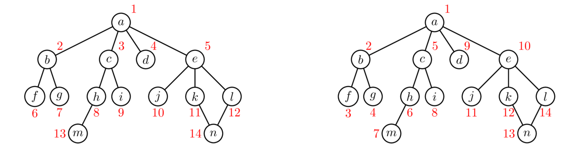
Notice how BFS works gradually outward from vertex a. Every vertex at distance 1 from a is visited before any vertex at distance 2, every vertex at distance 2 is visited before any vertex at distance 3, etc. DFS, on the other hand, follows a path down into the graph as far as it can go until it gets stuck. Then it backtracks to its previous location and tries searching from there some more. It continues this strategy of following paths and backtracking.

These are the two key ideas: BFS fans out from the starting vertex, doing a systematic sweep to deeper and deeper levels. DFS just goes as far down as it can go. When it can't go any further, it backs up a level and tries to explore other directions from that lavel. If we are just trying to find all the vertices in a graph, then both BFS and DFS will work equally well. However, if we are searching for vertices with a particular property, then depending on where those vertices are located in relation to the start vertex, BFS and DFS will behave differently. BFS, with its systematic search, will always find the closest vertex to the starting vertex. However, because of its systematic sweep, it might take BFS a while before it gets to vertices far from the starting vertex. DFS, on the other hand, can very quickly get far from the start, but will often not find the closest vertex first.

Code for BFS

In both BFS and DFS, we start at a given vertex and see what we can find from there. The searching process consists of visiting a vertex, looking at its neighbors, and adding any new neighbors to two separate lists. One list (actually a set) is for keeping track of what vertices we have already found. The other list keeps track of the order we will visit vertices to see what their neighbors are. Here is some code implementing BFS:

def bfs(G, start):
    found = {start}
    waiting = [start]

    while waiting:
        w = waiting.pop(0)
        for n in G[w]:
            if n not in found:
                found.add(n)
                waiting.append(n)
    return found

The function takes two parameters: a graph G and a vertex start, which is the vertex we start the search at. We maintain a set called found that remembers all the vertices we have found, and we maintain a list called waiting that keeps of the vertices we will be visiting. It acts like a queue. Initially, both start out with only start in them. We then continually do the following: pop off a vertex from the waiting list and loop through its neighbors, adding any neighbor we haven't already found into both the found set and waiting list. The while loop keeps running as long as the found list is not empty, i.e. as long as there are still vertices we haven't explored. At the end, we return all the vertices that were discovered by the search.

Let's run BFS on the graph below, starting at vertex a. The first thing the algorithm does is add each of the neighbors of a to the waiting list and waiting set. So at this point, the waiting list is [b, c, d, e]. BFS always visits the first vertex in the found list, so it visits b next and adds its neighbors to the list and set. So now the waiting list is [c, d, e, f, g]. For the next step, we take the first thing off the waiting list, which is c and visit it. We add its neighbors h and i to the list and set. This gives us a waiting list of [d, e, f, g, h, i]. As the process continues, the waiting list will start shrinking and the waiting set will eventually include all the vertices.

Here are several important notes about this code:

The code has been deliberately kept small. It has the effect of finding all the vertices that can be reached from the starting vertex. We will soon see how to modify this code to do more interesting things.
The method requires us to pass it a starting vertex. We could also use waiting as the first line, which will pick a vertex from the graph for us.
We could use a list for found instead of a set, but the result would be substantially slower for large graphs. The part where we check to see if a vertex is already in the v = next(iter(G)) set is the key. Python uses a O(1) hash-based approach to check if something is in a set, which is faster than the O(n) approach for checking a list.

Running time and memory usage

The running time is O(v+e), where v and $e are the number of vertices and edges, respectively, in the graph. The most edges we could have in a graph is v(v–1)/2, if every vertex is adjacent to every other vertex, so O(v+e) becomes O(v²) in that case. If we're searching a tree with depth d with each vertex having an average of b children, then the running time is O(b^d). This is important as one way to program artificial intelligence for games is to create a tree where the vertices are states of the game and edges go from the current state to all possible states you can get to by doing a legitimate move in the game. Often these trees will end up pretty deep, meaning BFS won't be able to search the whole tree in a reasonable amount of time. For instance, if there are 10 possible decisions at each point in a game that can take up to 50 turns, then BFS will need to investigate an unreasonable 10⁵⁰$ possible vertices to determine an optimal move.

The memory usage of BFS is O(v), which becomes O(b^d) in the tree case mentioned above. This can also become unreasonable when searching a deep tree.

Code for DFS

One way to implement DFS, it to use the exact same code as BFS except for one extremely small change: Use found instead of found. Everything else stays the same. Using waiting.pop() changes the order in how we choose which vertex to visit next. DFS visits the most recently added vertex, while BFS visits the earliest added vertex. BFS treats the list of vertices to visit as a queue, while DFS treats the list as a stack.

Though it works, it's probably not the best way to implement DFS. Recall that DFS works by going as down in the tree until it gets stuck, then backs up one step, tries going further along a different path until it gets stuck, backs up again, etc. One benefit of this approach is that it doesn't require too much memory. The search just needs to remember info about the path it is currently on. The approach described above, on the other hand, adds all the neighbors of a vertex into the waiting list as soon as it finds them. This means the waiting list can grow fairly large, like in BFS. Below is a different approach that avoids this problem.

def dfs(G, start):
    waiting = [start]
    found = {start}
    while waiting:
        w = waiting[-1]
        N = [n for n in G[w] if n not in found]
        if len(N) == 0:
            waiting.pop()
        else:
            n = N[0]
            found.add(n)
            waiting.append(n)
    return found

This code has running time O(v+e), just like BFS, but it's memory usage is better. In the case of a tree with depth d and branching factor b, BFS has space usage O(b^d), while this version of DFS has space usage O(bd), since it only has to remember info about the current path. This is a huge difference. The code above is also useful for certain algorithms that rely on the backtracking nature of DFS.

You'll often see DFS implemented recursively. It's probably more natural to implement it that way. Here is a short function to do just that:

def dfs(G, w, found):
    found.add(w)
    for x in G[w]:
        if x not in found:
            dfs(G, x, found)

We have to pass it a set to hold all the vertices it finds. For instance, if we're starting a search at a vertex labeled waiting.pop(0), we could create the set as waiting.pop() and then call 'a'.

Variations on the BFS and DFS algorithm

Returning a path

Here is a variation of BFS that finds the shortest path, in terms of least number of intermediate vertices, between a start and a goal vertex. The big change here is to turn the S = {'a'} set into a dictionary. When we find a new vertex, we use this dictionary to record what vertex's neighbors we were exploring when we found it. This allows us to remember each vertex's “parent” or immediate predecessor on the search. We can use this to create a path through the graph between the start and goal vertices. The code in the dfs(G, 'a', S) block uses this dictionary to trace back and return the path. Since we are using BFS, the path is guaranteed to be as short as possible.

def bfs_path(G, start, goal):
    found = {start:None}
    waiting = [start]

    while waiting:
        w = waiting.pop(0)
        for x in G[w]:
            if x == goal:
                path = [x]
                x = w
                while found[x] != None:
                    path.append(x)
                    x = found[x]
                path.append(x)
                path.reverse()
                return path

            if x not in found:
                found[x] = w
                waiting.append(x)
    return []

If we replace found with if x == goal, we would have a variation of DFS that returns a path. Unlike with BFS, there is no guarantee that the path returned by DFS will be the shortest one possible. Sometimes it is optimal, but quite often it is long and meandering.

Iterative deepening DFS

BFS is nice in that it will find the shortest path between the start and goal vertices. Its major flaw is that it can be a memory hog. It needs to hold a lot more things in its queue than DFS needs to hold in its stack. In particular, for a tree with d levels and branching factor b, BFS needs O(b^d) memory, while DFS only needs O(bd) memory. The downside of DFS is that it won't return optimal paths usually. But we can modify it in a way so that it will return an optimal path. The first step to doing this is to create a depth-limited version of DFS. For this, we simply put a limit to the search that doesn't let DFS get any more than a certain distance away from the start vertex. Here is the code:

def depth_limited_dfs(G, start, limit):
    waiting = [(start, 0)]
    found = {start}
    while waiting:
        w, current_depth = waiting[-1]
        if current_depth == limit:
            waiting.pop()
            continue
        N = [n for n in G[w] if n not in found]
        if len(N) == 0:
            waiting.pop()
        else:
            n = N[0]
            found.add(n)
            waiting.append((n, current_depth+1))
    return found

The main change to this over the earlier DFS code is to add a depth variable that gets put with each vertex on the waiting list. Each time we add a new thing to that list, we increase the depth level by 1, and if we hit the depth limit, then we don't add anything new from the vertices at that limit.

We can modify this into a search called iterative deepening. The idea is to run the depth-limited DFS with ever-increasing values of the depth. We start with depth 1, then depth 2, 3, 4, …. This guarantees we will find a shortest path. One obvious problem is we are repeating ourselves over and over again. For instance, all the work of the depth=3 search will be repeated when we do the depth=4 search. In many cases, the bulk of the work turns out to be at the deepest levels, so this repetition doesn't turn out to be such a bad thing. And remember that the benefit of doing this that we use much less memory than BFS. Below is the iterative deepening code, formulated to return the shortest path between the start and goal vertices.

def depth_limited_path(G, start, goal, limit):
    waiting = [(start, 0)]
    found = {start:None}
    while waiting:
        w, current_depth = waiting[-1]
        if current_depth == limit:
            waiting.pop()
            continue
        N = [n for n in G[w] if n not in found]
        if len(N) == 0:
            waiting.pop()
        else:
            n = N[0]
            found[n] = w
            if n == goal:
                path = []
                while found[n] != None:
                    path.append(n)
                    n = found[n]
                path.append(n)
                path.reverse()
                return path
            waiting.append((n, current_depth+1))
    return []

def iterative_deepening_path(G, start, goal, max_depth):
    for i in range(1, max_depth):
        result = depth_limited_path(G, start, goal, i)
        if result != []:
            return result

Applications of BFS and DFS

Word ladders

A word ladder is a type of puzzle where you are given two words and you have to get from one to another by changing a single letter at a time, with each intermediate word being a real word. For example, to get from time to rise, we could do time → tide → ride → rise.

We can model this as a graph whose vertices are words, with edges whenever two words differ by a single letter. Solving a word ladder amounts to finding a path in the graph between two vertices. Here is code that will create the graph using four-letter words. It relies on a wordlist file. Such files are freely available on the internet.

words = [line.strip() for line in open('wordlist.txt')]
words = set(w for w in words if len(w)==4)
alpha = 'abcdefghijklmnopqrstuvwxyz'

G = Graph()
for w in words:
    G.add(w)

for w in words:
    for i in range(len(w)):
        for a in alpha:
            n = w[:i] + a + w[i+1:]
            if n in words and n != w:
                G.add_edge(w, n)

The trickiest part of the code is the part that adds the edges. To do that, for each word in the list, we try changing each letter of the word to all possible other letters, and add an edge whenever the result is a real word. Once the graph is built, we can call one of the searches to find word ladders, like below:

print(bfs_path(G, 'wait', 'lift'))
print(iterative_deepening_path(G, 'wait', 'lift', 1000))

It's fun to try changing the BFS path approach to a DFS path approach (just modify the pop call in BFS). It finds word ladders, but they can come out dozens or even hundreds of words long. Many other puzzles and games can be solved by using a BFS or DFS approach like this.

Components

The basic versions of BFS and DFS that we presented return all the vertices in the same component as the starting vertex. With a little work, we can modify this to return a list of all the components in the graph. A graph's components are its “pieces.” Specifically, two vertices are in the same component if there is a way to get from one to another. They are in different components if there is no such path.

We can find components by looping over all the vertices in the graph and running a BFS or DFS using each vertex as a starting vertex. Of course, once we know what component a vertex belongs to, there is no sense in running a search from it, so in our code we'll skip vertices that we have already found. Here is the code:

def components(G):
    component_list = []
    found = set()
    for w in G:
        if w in found:  # skip vertices whose components we already know
            continue

        # now run a DFS starting from vertex w
        found.add(w)
        component = [w]
        waiting = [w]

        while waiting:
            v = waiting.pop()
            for u in G[v]:
                if u not in found:
                    waiting.append(u)
                    component.append(u)
                    found.add(u)
        component_list.append(component)
    return component_list

Here is code to call this on the word-ladder graph of 4-letter words:

L = sorted(components(G), key=len, reverse=True)
print([len(x) for x in L])

Here is the result:

[2485, 6, 5, 5, 4, 4, 3, 3, 3, 3, 3, 3, 3, 2, 2, 2, 2, 2, 2, 2, 2, 1, 1, 1, 1, 1,
1, 1, 1, 1, 1, 1, 1, 1, 1, 1, 1, 1, 1, 1, 1, 1, 1, 1, 1, 1, 1, 1, 1, 1, 1, 1, 1,
1, 1, 1, 1, 1, 1, 1, 1, 1, 1, 1, 1, 1, 1, 1, 1, 1, 1, 1, 1, 1, 1, 1, 1, 1, 1, 1,
1, 1, 1, 1, 1, 1, 1, 1, 1, 1, 1, 1, 1, 1, 1, 1, 1, 1, 1, 1, 1, 1, 1]

We see that there is one component that consists of most 4-letter words, a couple of smallish components, and many singletons. The 6-vertex component is waiting.pop(0). Some of the singletons are waiting.pop(), ['acne', 'acre', 'acme', 'ache', 'achy', 'ashy'], and rely. These are vertices of the graph that have no neighbors.

Floodfill

Floodfilling is a technique used in graphics and other settings where you want to fill a region with something. If you've ever played Minesweeper and clicked on the right spot, you can clear a wide area. Floodfill is used there. Floodfill is also used by the paint bucket icon in Microsoft Paint. We can use DFS or BFS to implement a floodfill. In the example below, we will assume that we have a rectangular grid of cells with some of them set to the hymn character and the rest to the liar character. The cells are on a grid with coordinates of the form (r, c) with (0, 0) being the upper left. The search starts at a user-specified coordinate where there is a - character, and it looks for all the other * characters it can reach from there. It replaces all of them with a special character. The - characters act sort of like walls. We can go around them, but not through them while we're filling. Here is the code:

def floodfill(board, start):
    waiting = [start]
    found = {start}

    while len(waiting) > 0:
        w = waiting.pop()
        for n in get_neighbors(w, board):
            if n not in found:
                r, c = n
                if board[r][c] == '-':
                    found.add(n)
                    waiting.append(n)
    return found

def get_neighbors(v, board):
    r, c = v
    N = [(r+1,c), (r-1,c), (r,c+1), (r,c-1)]
    return [(a,b) for a,b in N if 0<=a<len(board) and 0<=b<len(board[0])]

board = """
------****--**
---***-------*
---******--***
*********-****
*********-****
*********-----
--------------
-------*******"""
board = [list(b) for b in board[1:].split('\n')]

for r, c in floodfill(board, (1, 10)):
    board[r][c] = chr(9608)

for r in range(len(board)):
    for c in range(len(board[r])):
        print(board[r][c], end='')
    print()

Note the code doesn't actually create a graph object. The graph here is more implicit than explicit. The cells of the board act as the vertices. Instead of creating edges, we use the - function, which returns the neighbors of a given cell. This technique of not explicitly creating a graph can be useful, especially when the graph itself would be very large or when we likely won't need more than a small portion of the graph.

Mazes

DFS is particularly known as an algorithm to solve mazes. It can also be used to generate them. Below is a program that uses DFS to traverse a maze. You really should copy-paste it and run it. It graphically shows the path DFS takes, making it really clear how DFS tries paths and backtracks when it reaches dead ends.

from tkinter import *
from time import sleep

def maze(B, w, last, found):
        draw_to_screen(w, 'yellow')
        for x in get_neighbors(B, w):
            if is_goal(B, x) and x != w:
                draw_to_screen(x, 'yellow')
                return True
            if x not in found:
                found.add(x)
                draw_to_screen(w, 'red')
                is_done = maze(B, x, last, found)
                draw_to_screen(w, 'yellow')
                if is_done:
                    return True
            draw_to_screen(w, 'red')

def draw_to_screen(coord, color):
    r,c = coord
    canvas.create_rectangle(30*c+2, 30*r+2, 30*c+30, 30*r+30, fill=color)
    canvas.update()
    sleep(.3)

def is_goal(board, v):
    r,c = v
    N = [(r+1,c),(r-1,c),(r,c+1),(r,c-1)]
    for r,c in N:
        if r==-1 or c==-1 or r==len(board) or c==len(board[r]):
            return True
    return False

def get_neighbors(board, v):
    r,c = v
    N = [(r+1,c),(r-1,c),(r,c+1),(r,c-1)]
    return [(r,c) for (r,c) in N if 0<=r<len(board) and 0<=c<len(board[0]) and board[r][c]=='-']

def draw():
    for r in range(len(board)):
        for c in range(len(board[r])):
            canvas.create_rectangle(30*c+2, 30*r+2, 30*c+30, 30*r+30,
                                    fill='gray' if board[r][c]=='*' else 'white')

board ="""
***************
*----****-*--**
--**--***-**--*
*-*-*-****---**
***-----**-*-**
*****-**---*---
*-------**-*-**
****--*--*-*-**
**----**---****
***************"""
board = [list(b) for b in board[1:].split('\n')]
root = Tk()
canvas = Canvas(width=600, height=600, bg='white')
canvas.grid()
draw()
found = {(2,0)}
maze(board, (2,0), None, found)